

51
Q&As related to x3DNA-DSSR; an online community for DNA/RNA structural bioinformatics x3DNA-DSSR · w3DNA
 Show Posts
This section allows you to view all posts made by this member. Note that you can only see posts made in areas you currently have access to.
Netiquette · Download · News · Gallery · G-quadruplexes · DSSR-Jmol · DSSR-PyMOL · Video Overview · DSSR v2.5.4 (DSSR Manual) · Homepage
52
General discussions (Q&As) / MOVED: How to change the criteria of base pair
« on: July 27, 2016, 06:55:00 pm »53
General discussions (Q&As) / MOVED: global bending of a single stranded DNA
« on: July 18, 2016, 04:46:34 pm »54
General discussions (Q&As) / How to setup 3DNA
« on: May 05, 2016, 02:24:00 pm »
Follow the instructions on "How to install 3DNA on Linux (Mac OS X) and Windows?" and post back any questions you may have.
Enjoy using 3DNA!
Xiang-Jun
Enjoy using 3DNA!
Xiang-Jun
55
Site announcements / Summary of registrations
« on: April 26, 2016, 03:25:27 pm »
Since the current 3DNA Forum (using SMF in place of the initial phpBB) was started in early 2012, it has attracted 2,750+ registrants as of today (April 26, 2016). Over the past four years, there are around 50 new registrations per month, or ~600 per year, as shown below:
If the current trend continues, the number of 3DNA Forum registered users will reach 3,000 by the end of September 2016. Overall, the Forum has fulfilled its intended goals on "Q&As related to 3DNA" and serving as "an online community for DNA/RNA structural bioinformatics."
A large number of the registrants use their work email addresses (e.g., .edu), in line with the trust the community has gradually put on the 3DNA Forum. For example, over half of this month's 62 registrations (as of this writing, 2016-04-26) are filled with clearly identifiable job-related emails. Of course, personal emails (e.g., gmail, yahoo mail, qq.com or 163.com from China) are perfectly fine for registration with this Forum. Whatever the case, users information is kept confidential. Over the past four years, I remember having only sent two DSSR-related newsletters to all members.
Throughout the time, I've committed to a zero-tolenance policy on spams of various types. As a result, the Forum has remained spam free. Most legitimate registrations are activated automatically, and new users can gain immediate access to the download page. Occasionally, however, the anti-spam software blocks suspicious registrations even with .edu email accounts. In such rare cases, I am quick to verify/activate them manually, and notify the effected users by email. Of course, this process may take hours, depending on your time zone.
Code: [Select]
2012 -- 601
2013 -- 667
2014 -- 696
2015 -- 598
If the current trend continues, the number of 3DNA Forum registered users will reach 3,000 by the end of September 2016. Overall, the Forum has fulfilled its intended goals on "Q&As related to 3DNA" and serving as "an online community for DNA/RNA structural bioinformatics."
A large number of the registrants use their work email addresses (e.g., .edu), in line with the trust the community has gradually put on the 3DNA Forum. For example, over half of this month's 62 registrations (as of this writing, 2016-04-26) are filled with clearly identifiable job-related emails. Of course, personal emails (e.g., gmail, yahoo mail, qq.com or 163.com from China) are perfectly fine for registration with this Forum. Whatever the case, users information is kept confidential. Over the past four years, I remember having only sent two DSSR-related newsletters to all members.
Throughout the time, I've committed to a zero-tolenance policy on spams of various types. As a result, the Forum has remained spam free. Most legitimate registrations are activated automatically, and new users can gain immediate access to the download page. Occasionally, however, the anti-spam software blocks suspicious registrations even with .edu email accounts. In such rare cases, I am quick to verify/activate them manually, and notify the effected users by email. Of course, this process may take hours, depending on your time zone.
56
General discussions (Q&As) / Install 3DNA on Windows via MinGW/MSYS
« on: March 06, 2016, 08:46:19 pm »
Again, thanks for your persistence. In the end, you may find the learning experience well worth it!
3DNA should work if you have installed MinGW/MSYS properly. Given the difficult you experienced with installing Cygwin, let's focus on MinGW/MSYS. To get you up and running ASAP, please answer the following questions:
Xiang-Jun
3DNA should work if you have installed MinGW/MSYS properly. Given the difficult you experienced with installing Cygwin, let's focus on MinGW/MSYS. To get you up and running ASAP, please answer the following questions:
- Which version of Windows are you using?
- Where have you put the 3DNA v2.3 download (i.e. file x3dna-v2.3-mingw-win.tar.gz)?
- Have you extracted the tarball file into its folder x3dna-v2.3?
- In your MinGW/MSYS shell, what do you get with the command: "tar"?
Xiang-Jun
57
Site announcements / CCN short communication on base-pair geometry
« on: February 06, 2016, 10:57:25 am »
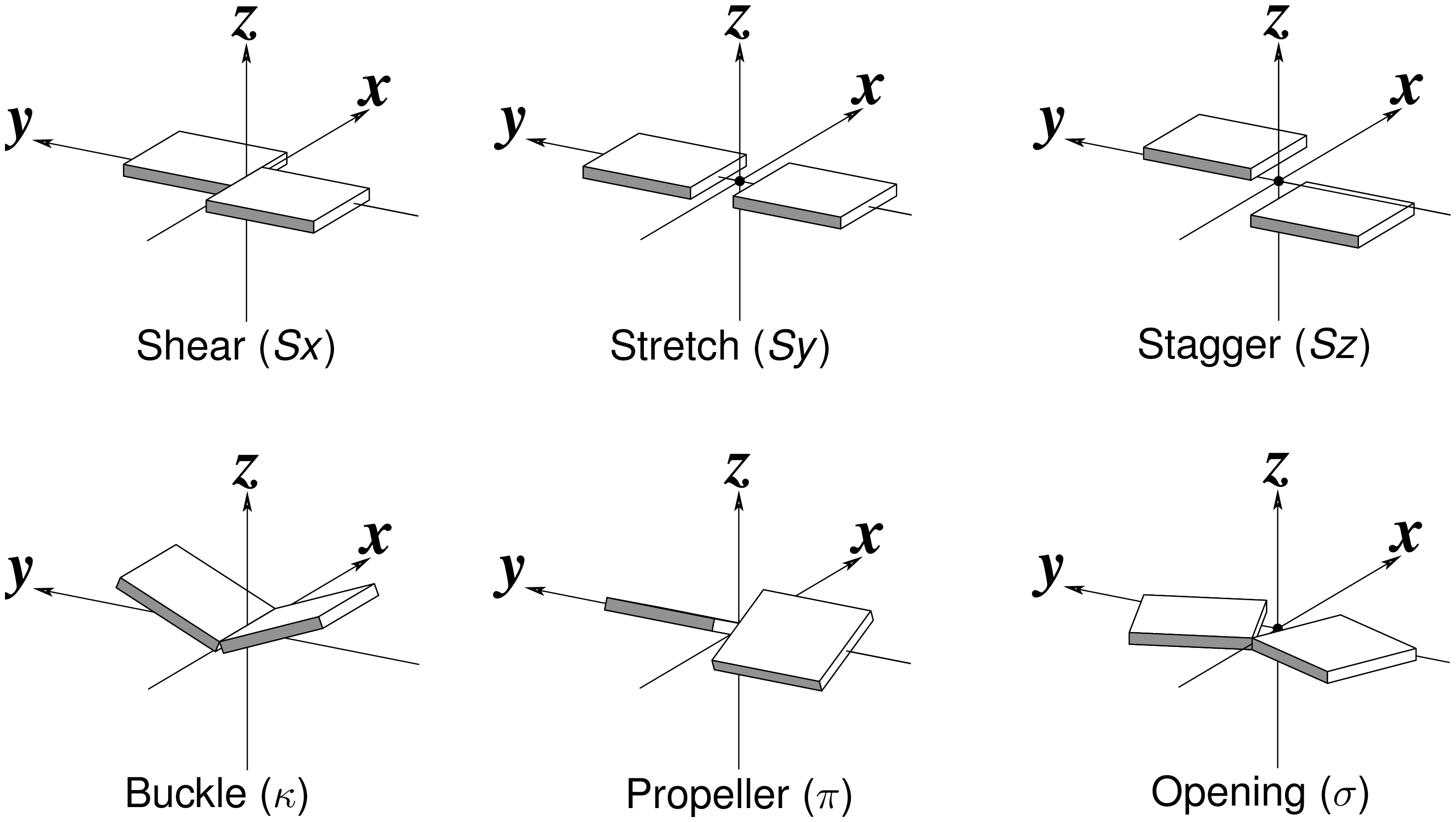
The 2016 January issue of the Computational Crystallography Newsletter (CCN) contains a short communication titled "Characterization of base pair geometry" (p.5-8) by Dr. Wilma Olson and me. This essay had been mostly motivated by two publications in the 2015 July issue of CCN by Dr. Jane Richardson: an article titled "A context-sensitive guide to RNA & DNA base pair & base-stack geometry," and an 'Expert advice' of 'Fitting Tip #10' titled "How do your base pairs touch and twist?" In both pieces, Richardson emphasized the importance of base-pair (bp) non-planarity introduced by Buckle and Propeller (see Figure below) for improved fit of DNA/RNA models to X-ray electron density maps. I derived a complete set of six simple bp parameters for a complete qualitative description of bp geometry. The term 'simple' is used because the parameters are more intuitive for non-canonical pairs, and to differentiate them from the existing local bp parameters in 3DNA.
In the CCN short communication, we also highlighted the DSSR-introduced cartoon-block representations of DNA and RNA structures that combine PyMOL cartoon schematics with color-coded rectangular base blocks (See Figure below). The simple, informative cartoon-block representations facilitate understanding of the base interactions in small to mid-sized nucleic acid structures where the base identity, pairing geometry, and stacking interactions are immediately obvious.
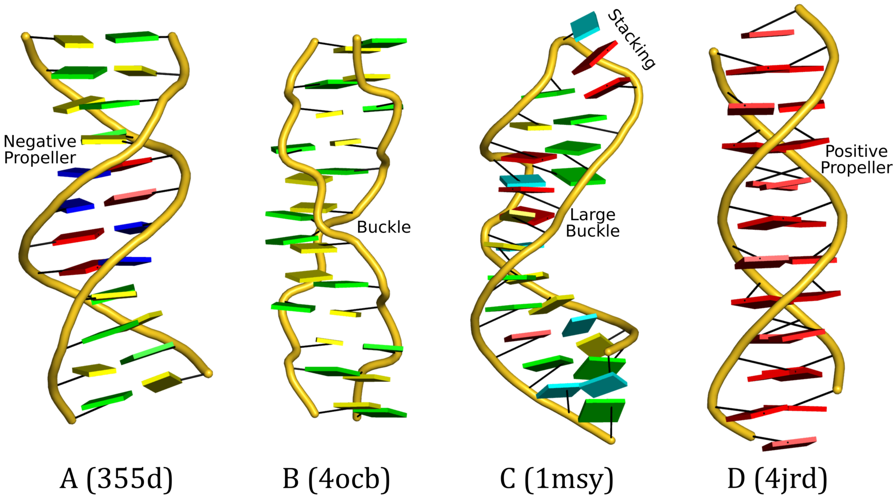
A blogpost with the same title "Characterization of base-pair geometry" contains details for reproducing the cartoon-block images in the figure above. See also links therein for further information.
Xiang-Jun
In the CCN short communication, we also highlighted the DSSR-introduced cartoon-block representations of DNA and RNA structures that combine PyMOL cartoon schematics with color-coded rectangular base blocks (See Figure below). The simple, informative cartoon-block representations facilitate understanding of the base interactions in small to mid-sized nucleic acid structures where the base identity, pairing geometry, and stacking interactions are immediately obvious.
A blogpost with the same title "Characterization of base-pair geometry" contains details for reproducing the cartoon-block images in the figure above. See also links therein for further information.
Xiang-Jun
58
Site announcements / Alternative 3DNA homepage at URL home.x3dna.org
« on: October 11, 2015, 01:37:43 pm »
In addition to the well-known 3DNA homepage at URL http://x3dna.org, I've recently duplicated its contents to an alternative site at http://home.x3dna.org. Hosted at Columbia University, the alternative homepage is accessible from countries like mainland China.
Over the years, I've heard of many times from potential 3DNA users in China who cannot visit http://x3dna.org which is on a shared host. Now http://home.x3dna.org, the 3DNA Forum (http://forum.x3dna.org), and a few other 3DNA/DSSR-related web services are all hosted on dedicated servers under my desk. They should be universally reachable.
Web-based technologies (on both the server and client sides) are now matured enough to make writing web applications enjoyable. The infrastructure in place makes it feasible to add more web-based functionality. Moreover, existing web services will be consolidated and refined to ensure sustainability and wide accessibility of 3DNA.
Xiang-Jun
59
Bug reports / MOVED: NUPARM vs 3DNA
« on: October 09, 2015, 12:45:24 pm »
This topic has been moved to General discussions (Q&As).
http://forum.x3dna.org/index.php?topic=581.0
http://forum.x3dna.org/index.php?topic=581.0
60
Site announcements / The Forum was down due to a power failure
« on: October 05, 2015, 11:49:39 am »
While at a meeting during the week (Oct. 2-4, 2015), I noticed that the Forum was suddenly out of service. Further explorations showed that several other websites and the DSSR manual were all not accessible. I suspected a power failure that had brought down the two servers (named x3dna and dssr) under my desk.
When I came to office this morning, I immediately found that both of my machines were off. Simply switching them on, and everything is back to normal. This is the first power failure experience after the x3dna and dssr servers have been put into service. Yet, it does remind me to have a backup plan.
Sorry for the inconvenience the shutdown may have caused.
Xiang-Jun
61
w3DNA -- web interface to 3DNA / MOVED: 3DNA can recognise DNA with S atoms?
« on: September 24, 2015, 11:31:04 pm »
This topic has been moved to General discussions (Q&As).
http://forum.x3dna.org/index.php?topic=577.0
http://forum.x3dna.org/index.php?topic=577.0
62
RNA structures (DSSR) / MOVED: Dinucleotide step parameters for "ideal" A-form RNA
« on: September 11, 2015, 03:52:08 pm »
This topic has been moved to General discussions (Q&As).
http://forum.x3dna.org/index.php?topic=575.0
http://forum.x3dna.org/index.php?topic=575.0
63
DSSR-NAR paper / RNA cartoon-block representations with PyMOL and DSSR
« on: July 24, 2015, 02:18:56 pm »
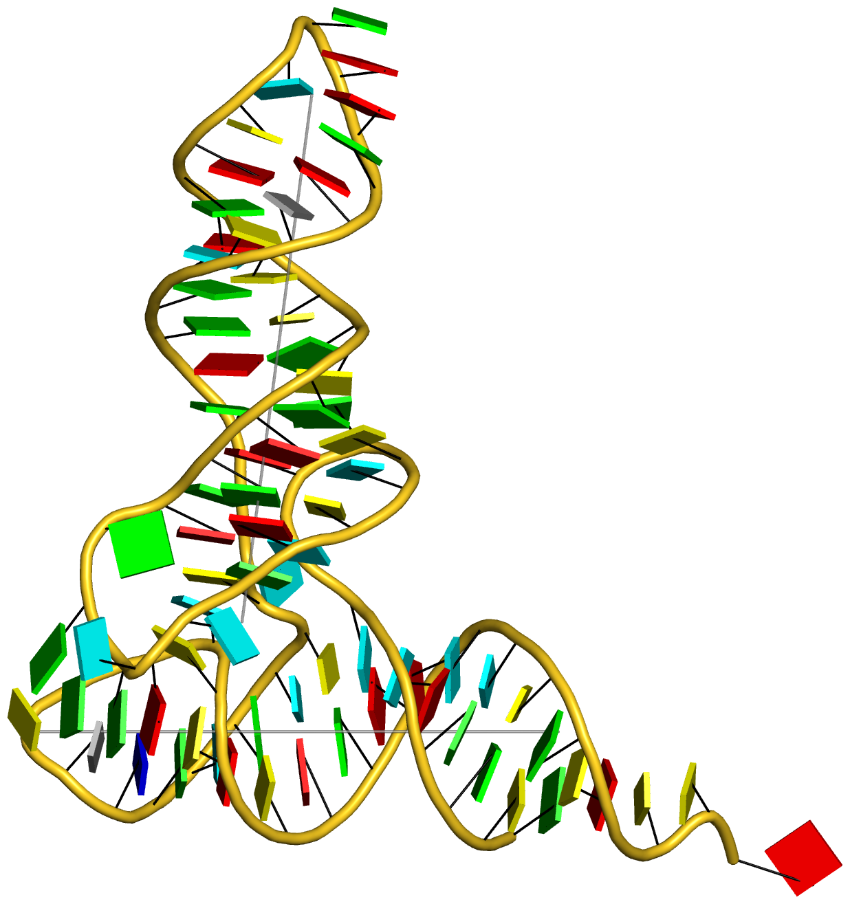
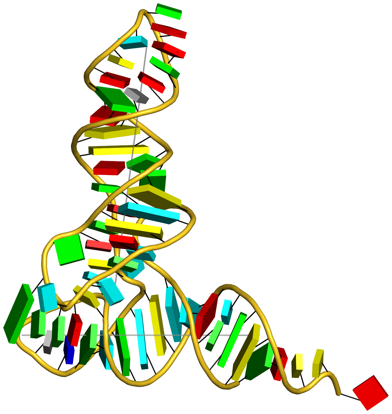
In addition to its functionality for RNA structural analysis, the DSSR program also introduces novel cartoon-block schematic representations of nucleic acid structures to be rendered with PyMOL. Illustrated below are four sample images with the script and all data files (cartoon-block.tar.gz).
Here is the script (named tasks in the associated tarball cartoon-block.tar.gz):
Following the above instructions, one should be able to reproduce the four sample images without a problem. Similar procedures can be easily applied to any other nucleic acid structures. Hopefully, this schematic visualization feature provides yet another reason for you to give DSSR a try.
Thomas Holder, the Principal Developer of PyMOL, has written a PyMOL plugin that implements the dssr_block command. Now users can create "block" shaped cartoons for nucleic acid bases and base pairs interactively in PyMOL.
Note added on 2016-04-01: DSSR now also has two new related options, --cartoon-block and --block-color, to make the generation of schematic cartoon block images more straightforward, and flexible.
 |  |
 |  |
Here is the script (named tasks in the associated tarball cartoon-block.tar.gz):
Code: Bash
- # ------------------------------------------------------------------
- # 1. Yeast phenylalanine tRNA 1ehz in default settings.
- # Note the coordinates ("1ehz-ok.pdb") is transformed from the
- # original PDB file "1ehz.pdb" to put the helix containing the T-stem
- # and acceptor stem horizontally, and the helix containing the D-stem
- # and anti-codon stem 'vertically'.
- x3dna-dssr -i=1ehz-ok.pdb --helical-axis -o=temp # note the --helical-axis option
- \mv dssr-helicalAxes.pdb 1ehz-ok-helices.pdb # rename file with helical axes
- x3dna-dssr -i=1ehz-ok.pdb --block-file -o=1ehz-ok-blocks.r3d # note the option --block-file
- # The three files "1ehz-ok.pdb", "1ehz-ok-blocks.r3d", and
- # "1ehz-ok-helices.pdb" combined in "1ehz-ok.pml" and ray-traced with
- # PyMOL to get "1ehz-ok-pymol.png".
- pymol -qkc 1ehz-ok.pml
- convert -trim +repage -border 10 -bordercolor white 1ehz-ok-pymol.png 1ehz-ok.png # just to crop
- # ------------------------------------------------------------------
- # 2. tRNA 1ehz with thicker rectangular blocks and Watson-Crick bps in
- # longer blocks.
- \cp 1ehz-ok.pdb 1ehz-wc.pdb # just give it a different name
- x3dna-dssr -i=1ehz-wc.pdb --helical-axis -o=temp
- \mv dssr-helicalAxes.pdb 1ehz-wc-helices.pdb
- x3dna-dssr -i=1ehz-wc.pdb --block-file=wc --block-depth=1.2 -o=1ehz-wc-blocks.r3d
- # Note the options "--block-file=wc" and "--block-depth=1.2". The
- # default block thickness (depth) is 0.5 angstrom. Again, file
- # "1ehz-wc.pml" combines the components to be ray-traced by PyMOL.
- pymol -qkc 1ehz-wc.pml
- convert -trim +repage -border 10 -bordercolor white 1ehz-wc-pymol.png 1ehz-wc.png
- # ------------------------------------------------------------------
- # 3. GUAA tetraloop mutant of sarcin/ricin domain from E. Coli 23S
- # rRNA -- 1msy, with minor groove in black and oriented in a bp
- # reference frame.
- x3dna-dssr -i=1msy.pdb --frame=A.2658+edge+wc -o=1msy-ok.pdb # set the view
- x3dna-dssr -i=1msy-ok.pdb -o=temp
- x3dna-dssr -i=1msy-ok.pdb --block-file=minor+wc --block-depth=0.8 -o=1msy-ok-blocks.r3d
- # Note the options "--frame=A.2658+edge+wc" and
- # "--block-file=minor+wc".
- # The "1msy-ok.pml" file is for PyMOL rendering.
- pymol -qkc 1msy-ok.pml
- convert -trim +repage -border 10 -bordercolor white 1msy-ok-pymol.png 1msy-ok.png
- # ------------------------------------------------------------------
- # 4. 1msy, with blocks in outline mode.
- \cp 1msy-ok.pdb 1msy-edge.pdb
- x3dna-dssr -i=1msy-edge.pdb -o=temp
- x3dna-dssr -i=1msy-edge.pdb --block-file=edge -o=1msy-edge-blocks.r3d
- # Note the option "--block-file=edge", and file "1msy-edge.pml".
- pymol -qkc 1msy-edge.pml
- convert -trim +repage -border 10 -bordercolor white 1msy-edge-pymol.png 1msy-edge.png
Following the above instructions, one should be able to reproduce the four sample images without a problem. Similar procedures can be easily applied to any other nucleic acid structures. Hopefully, this schematic visualization feature provides yet another reason for you to give DSSR a try.
Thomas Holder, the Principal Developer of PyMOL, has written a PyMOL plugin that implements the dssr_block command. Now users can create "block" shaped cartoons for nucleic acid bases and base pairs interactively in PyMOL.
Note added on 2016-04-01: DSSR now also has two new related options, --cartoon-block and --block-color, to make the generation of schematic cartoon block images more straightforward, and flexible.
64
Site announcements / The DSSR paper has been published in Nucleic Acids Research
« on: July 17, 2015, 02:25:03 pm »
After numerous efforts, it is a real pleasure to see the publication of the paper titled "DSSR: an integrated software tool for dissecting the spatial structure of RNA" in Nucleic Acids Research.
Here is the abstract:
While only time can tell the impact of a scientific contribution, I feel confident to predict that, in the long run, the DSSR paper will receive many more citations than the 3DNA papers combined. With a unique balance of the description of novel methods and the illustrated new findings enabled by the software, the DSSR paper stands clearly at the very top among all my publications. I am also completely satisfied with the editing outcome in the final page-proof stage (going through three iterations, on issues of deleting a comma, changing dash–to-hyphen etc) before it is finalized for publication.
For those who are interested in details, I have added a new section titled "DSSR-NAR paper" with scripts and related data files for the reproduction of our reported results. As always, I welcome any comments, and I strive to respond promptly to each and every question you may have on the DSSR paper.
Xiang-Jun
Here is the abstract:
Quote
Insight into the three-dimensional architecture of RNA is essential for understanding its cellular functions. However, even the classic transfer RNA structure contains features that are overlooked by existing bioinformatics tools. Here we present DSSR (Dissecting the Spatial Structure of RNA), an integrated and automated tool for analyzing and annotating RNA tertiary structures. The software identifies canonical and noncanonical base pairs, including those with modified nucleotides, in any tautomeric or protonation state. DSSR detects higher-order coplanar base associations, termed multiplets. It finds arrays of stacked pairs, classifies them by base-pair identity and backbone connectivity, and distinguishes a stem of covalently connected canonical pairs from a helix of stacked pairs of arbitrary type/linkage. DSSR identifies coaxial stacking of multiple stems within a single helix and lists isolated canonical pairs that lie outside of a stem. The program characterizes ‘closed’ loops of various types (hairpin, bulge, internal, and junction loops) and pseudoknots of arbitrary complexity. Notably, DSSR employs isolated pairs and the ends of stems, whether pseudoknotted or not, to define junction loops. This new, inclusive definition provides a novel perspective on the spatial organization of RNA. Tests on all nucleic acid structures in the Protein Data Bank confirm the efficiency and robustness of the software, and applications to representative RNA molecules illustrate its unique features. DSSR and related materials are freely available at http://x3dna.org/.
While only time can tell the impact of a scientific contribution, I feel confident to predict that, in the long run, the DSSR paper will receive many more citations than the 3DNA papers combined. With a unique balance of the description of novel methods and the illustrated new findings enabled by the software, the DSSR paper stands clearly at the very top among all my publications. I am also completely satisfied with the editing outcome in the final page-proof stage (going through three iterations, on issues of deleting a comma, changing dash–to-hyphen etc) before it is finalized for publication.
For those who are interested in details, I have added a new section titled "DSSR-NAR paper" with scripts and related data files for the reproduction of our reported results. As always, I welcome any comments, and I strive to respond promptly to each and every question you may have on the DSSR paper.
Xiang-Jun
65
DSSR-NAR paper / Figure 6 -- analysis of the CRISPR Cas9-sgRNA-DNA ternary complex (4oo8)
« on: July 08, 2015, 08:46:35 pm »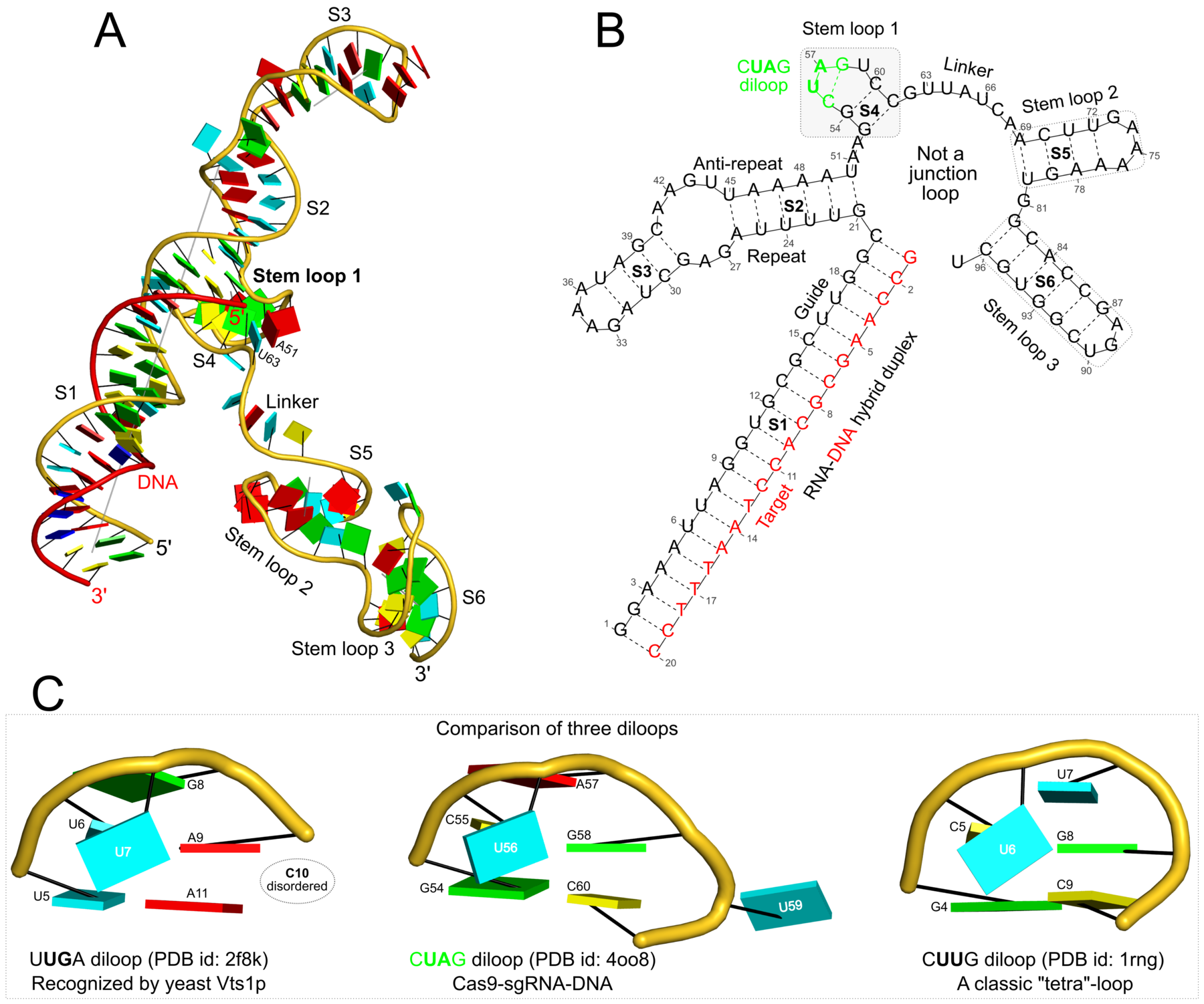
Quote
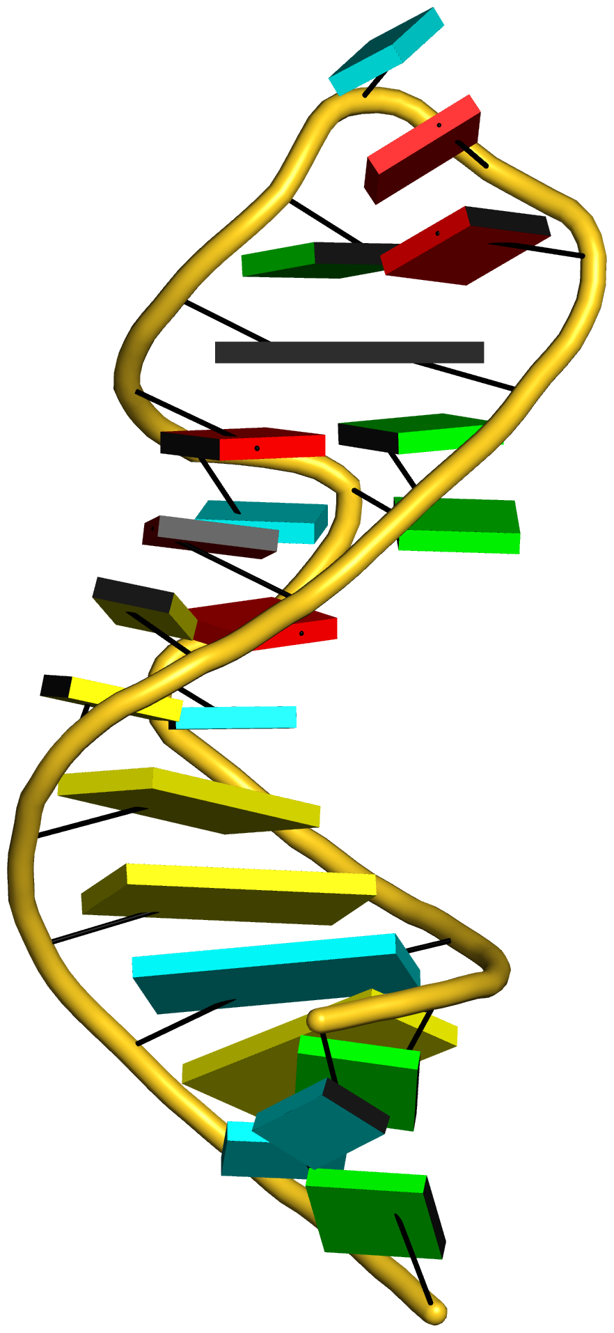
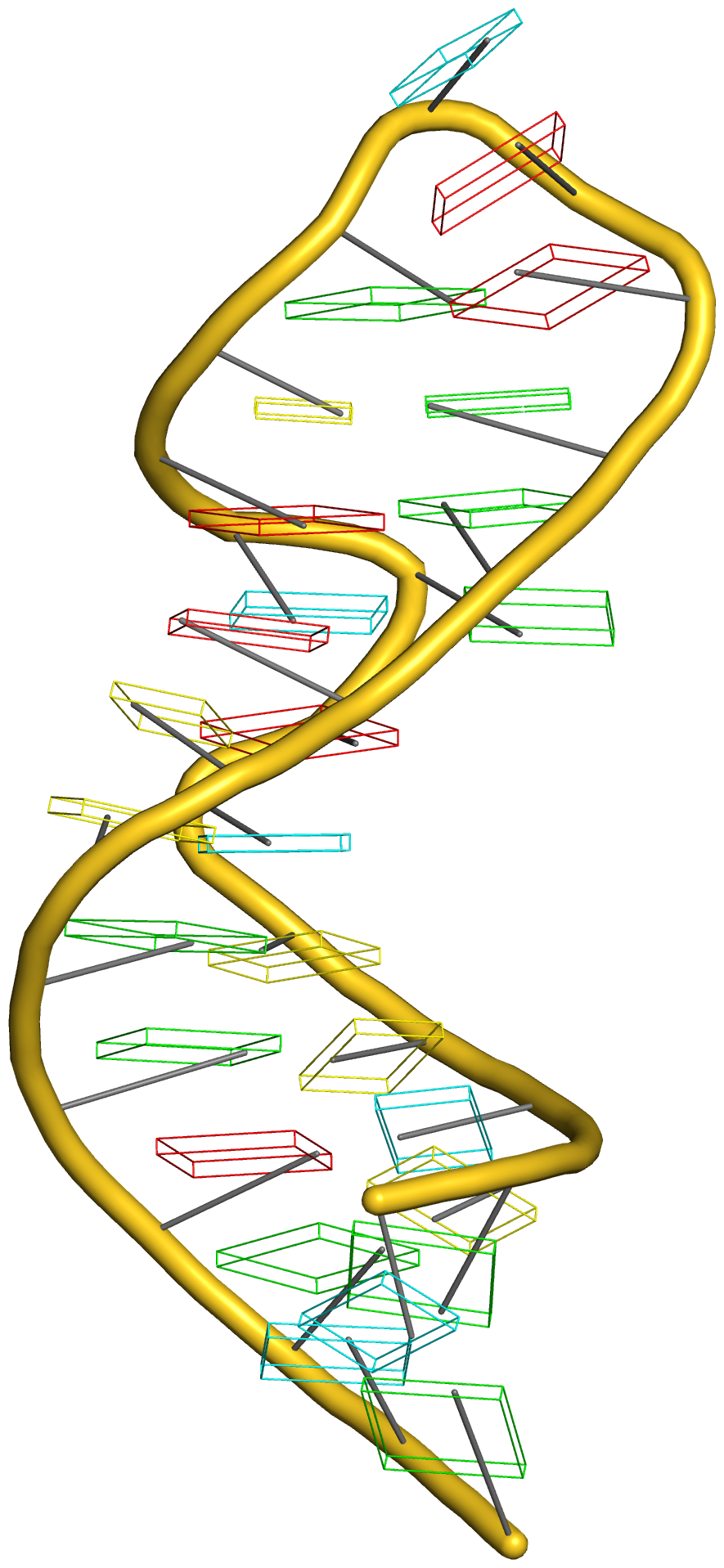
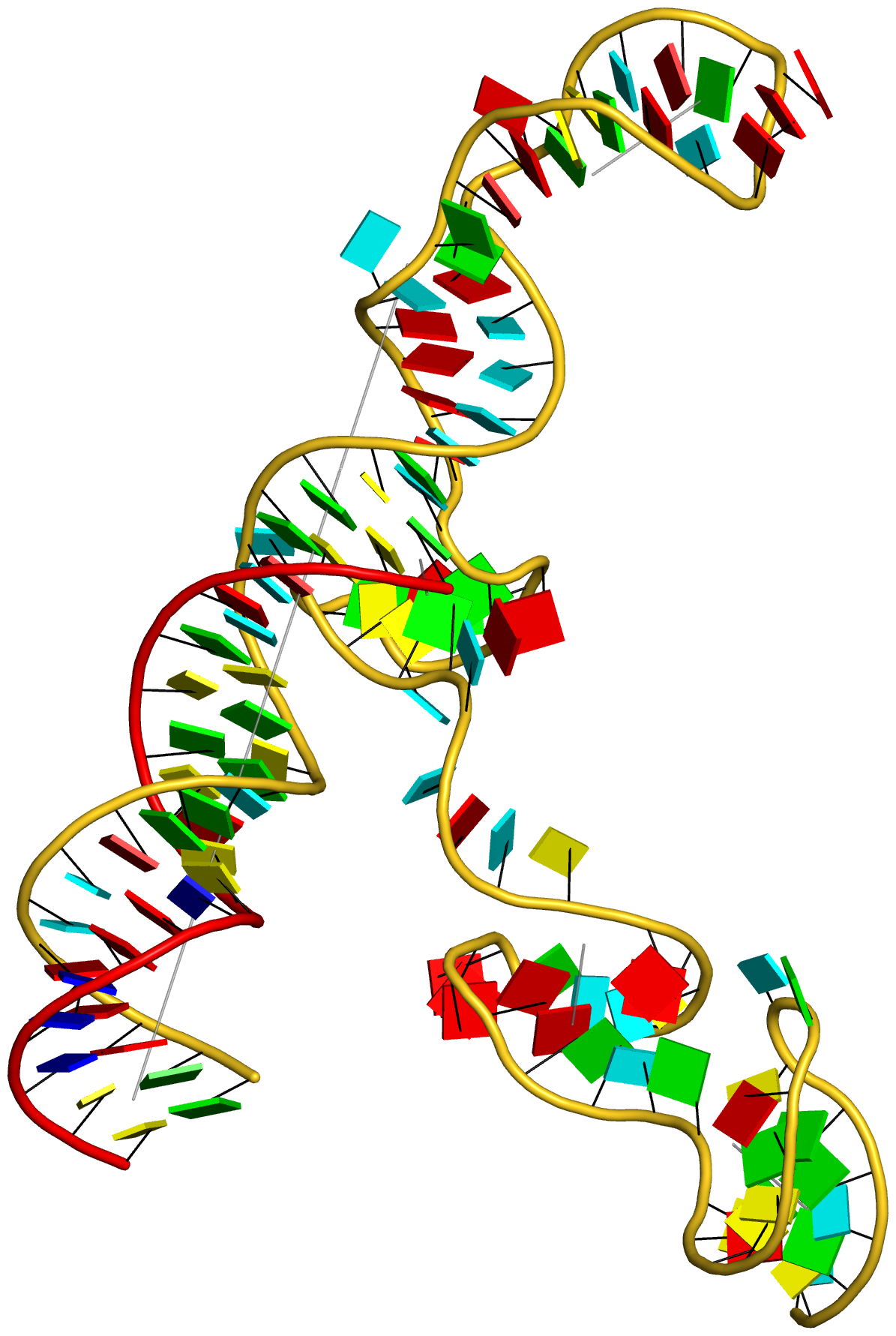
Figure 6: DSSR applies to RNA-DNA hybrid structures, such as the CRISPR Cas9-sgRNA-DNA ternary complex (chains B and C, PDB id: 4oo8 (47)). (A) The software identifies five helices (depicted by gray lines) and six stems (annotated) in the structure. The longest helix includes the RNA-DNA hybrid duplex (S1, depicted by intertwined gold-red backbone tubes) and the repeat:anti-repeat RNA stem (S2). (B) The secondary structure diagram, derived using DSSR, shows that the hybrid structure does not form a ‘closed’ junction loop. DSSR classifies the CUAG hairpin loop as a diloop (instead of a tetraloop) because the C and G form a Watson-Crick pair that closes the loop, leaving only a two-nucleotide (UA) loop segment. (C) Comparison of the CUAG diloop (center) with the UUGA diloop from a yeast Vts1p-RNA hairpin complex (referred to as part of a pentaloop(59), left) shows the remarkable similarity between the two loops despite the large difference in their base sequences. The CUAG diloop also shares common features with the NMR solution structure of the classic CUUG diloop(60) (often called a tetraloop, right), including the flipped out second position U and the stacking of the closing C–G pair over a neighboring G–C pair. The diloops differ, however, in terms of the inter-pair twist angle at the GpC dinucleotide step. These three images are oriented in the frames of the purines stacked above the terminal nucleotides (A9-left; G58-middle; G8-right) with the minor-groove edges facing the viewer.
Here is the tarball (fig6-CRISPR-Cas9-4oo8.tar.gz) with the script and all related data files.
The content of the full script (named tasks) is shown below. Please see also notes for "Figure 2 -- analysis of the yeast phenylalanine tRNA (1ehz)".
Code: Bash
- # Step #1 -- reorient CRISPR-Cas9 RNA-DNA hybrid into the most extended view
- pdb_frag B 1:97 C 1:20 4oo8.pdb 4oo8-nts.pdb
- rotate_mol 4oo8-nts.pdb temp
- rotate_mol -r=4oo8.rot temp 4oo8-ok.pdb
- x3dna-dssr -i=4oo8-ok.pdb --prefix=4oo8-ok -o=4oo8-ok.out
- # To get the result illustrated in panel B, load '4oo8-ok-2ndstrs.ct'
- # or '4oo8-ok-2ndstrs.dbn' into VARNA to draw the planar secondary
- # structure diagram, exported as .svg for annotation in Inkscape.
- # Step #2 -- get the cartoon-block representation, with fitted helices
- x3dna-dssr -i=4oo8-ok.pdb --helical-axis -o=temp
- \mv dssr-helicalAxes.pdb 4oo8-ok-helices.pdb
- x3dna-dssr -i=4oo8-ok.pdb --block-file -o=4oo8-ok-blocks.r3d
- # see 4oo8-ok.pml -- panel A
- pymol -qkc 4oo8-ok.pml
- convert -trim +repage -border 10 -bordercolor white 4oo8-ok-pymol.png 4oo8-ok.png
- # Step #3 -- comparison of diloops (panel C)
- pdb_frag B 5:11 2f8k.pdb temp
- x3dna-dssr -i=temp --frame=B.9:edge -o=temp2
- rotate_mol -r=rotxy-180 temp2 2f8k-uuga.pdb
- x3dna-dssr -i=2f8k-uuga.pdb --block-file -o=2f8k-uuga-blocks.r3d
- # see file: 2f8k-uuga.pml
- pymol -qkc 2f8k-uuga.pml
- convert -trim +repage -border 10 -bordercolor white 2f8k-uuga-pymol.png 2f8k-uuga.png
- pdb_frag B 54:60 4oo8-ok.pdb temp
- x3dna-dssr -i=temp --frame=B.58:edge -o=temp2
- rotate_mol -r=rotxy-180 temp2 4oo8-cuag.pdb
- x3dna-dssr -i=4oo8-cuag.pdb --block-file -o=4oo8-cuag-blocks.r3d
- # see file: 4oo8-cuag.pml
- pymol -qkc 4oo8-cuag.pml
- convert -trim +repage -border 10 -bordercolor white 4oo8-cuag-pymol.png 4oo8-cuag.png
- ex_str -1 1rng.pdb model1.pdb
- pdb_frag A 4:9 model1.pdb temp
- x3dna-dssr -i=temp --frame=A.8:edge -o=temp2
- rotate_mol -r=rotxy-180 temp2 1rng-cuug.pdb
- x3dna-dssr -i=1rng-cuug.pdb --block-file -o=1rng-cuug-blocks.r3d
- # see file: 1rng-cuug.pml
- pymol -qkc 1rng-cuug.pml
- convert -trim +repage -border 10 -bordercolor white 1rng-cuug-pymol.png 1rng-cuug.png
Here are the images generated from the above script:
66
DSSR-NAR paper / Figure 5 -- analysis of the SAM-I riboswitch (2gis)
« on: July 08, 2015, 08:43:50 pm »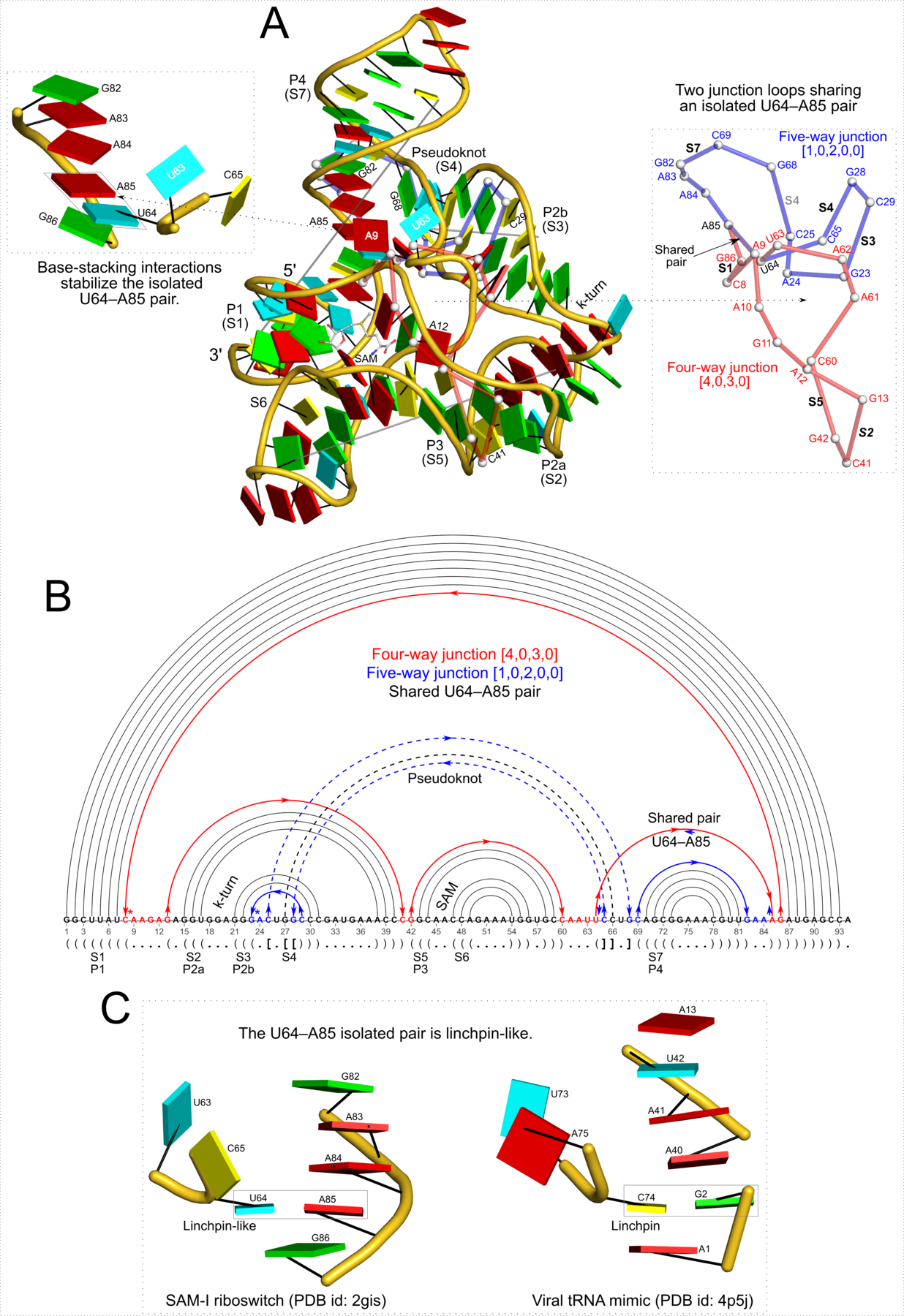
Quote
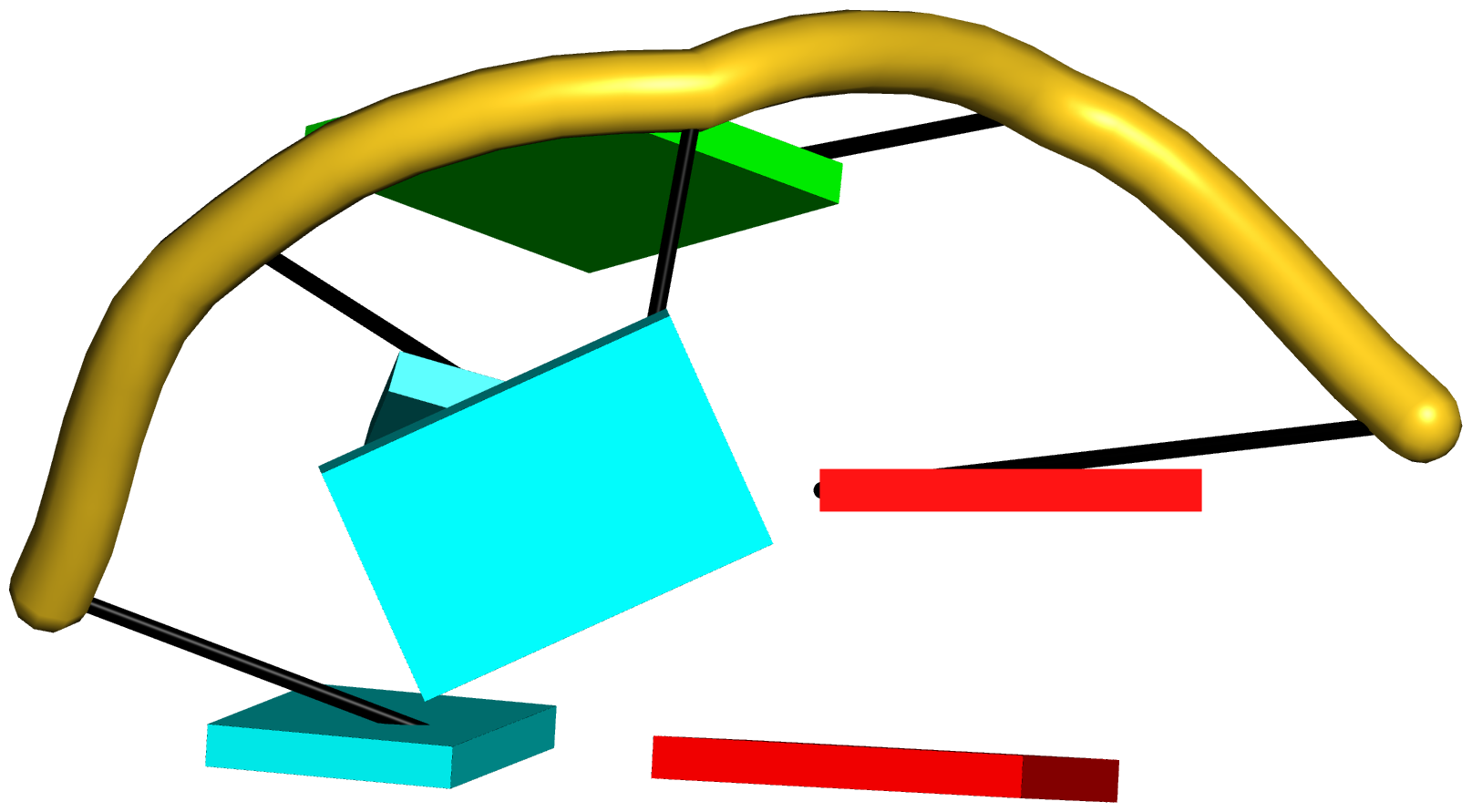
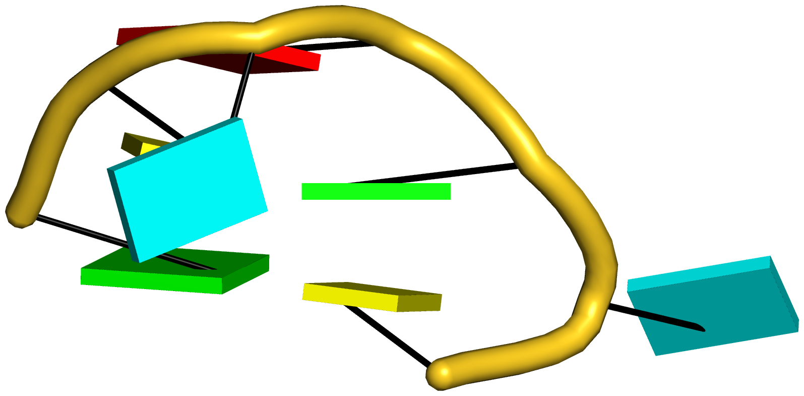
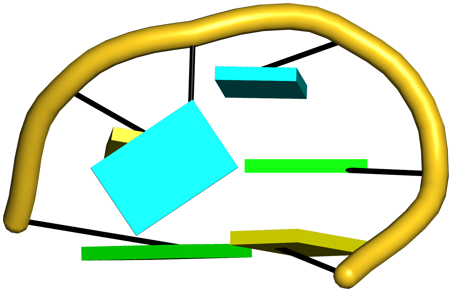
Figure 5: DSSR pinpoints a linchpin-like U64–A85 pair that is shared by a four-way and a five-way junction loop in the S-adenosyl methionine I riboswitch (PDB id: 2gis (45)). (A) DSSR identifies two junction loops (right): a [4,0,3,0] four-way junction loop (red) and a [1,0,2,0,0] five-way junction loop (blue), which share a common side, i.e., the isolated U64–A85 pair (left). (B) The linear secondary structure diagram, annotated with DSSR-derived dot-bracket notation, depicts the pathways of the two junction loops. The four-way loop runs from C8 (*), follows the red arrows to the right, and returns along the outer G86→C8 arc. The five-way loop starts at G23 (*), moves to the right following the blue arrows along two arcs (C25→G68 and C69→G82), and returns to the start along three arcs (A85→U64, C65→G28, C29→G23). Note that the shared U64–A85 arc is traversed twice, from left to right along the four-way junction loop, and right to left along the five-way junction loop. (C) The U64–A85 pair is stabilized by base-stacking interactions in a way strikingly similar to the G2–C74 linchpin pair in the viral tRNA mimic (see Figure 3), and may also be regarded as a ‘linchpin’. These two images take advantage of unique visualization features within 3DNA/DSSR, including the capability to orient different molecules in a common frame (here, the frames of the linchpin pairs with the minor-groove edges facing the viewer) and to represent bases as color-coded rectangular blocks.
Here is the tarball (fig5-SAM-I-2gis.tar.gz) with the script and all related data files.
The content of the full script (named tasks) is shown below. Please see also notes for "Figure 2 -- analysis of the yeast phenylalanine tRNA (1ehz)".
Code: Bash
- # Step #1 -- reorient SAM-I riboswitch into the most extended view
- pdb_frag A 1:94 A 301 2gis.pdb 2gis-nts.pdb
- rotate_mol 2gis-nts.pdb temp
- rotate_mol -r=2gis.rot temp 2gis-ok.pdb
- x3dna-dssr -i=2gis-ok.pdb --prefix=2gis-ok -o=2gis-ok.out
- # To get the result illustrated in panel B, load '2gis-ok-2ndstrs.ct'
- # or '2gis-ok-2ndstrs.dbn' into VARNA to draw the linear secondary
- # structure diagram, exported as .svg for annotation in Inkscape.
- # Step #2 -- get the cartoon-block representation, with fitted helices
- x3dna-dssr -i=2gis-ok.pdb --helical-axis -o=temp
- \mv dssr-helicalAxes.pdb 2gis-ok-helices.pdb
- x3dna-dssr -i=2gis-ok.pdb --block-file -o=2gis-ok-blocks.r3d
- # Step #3 -- simplified representation of the [4,0,3,0] 4-way
- # and [1,0,2,0,0] 5-way junctions in 3D
- # note the '--raw-xyz' option: it keeps the original coordinates
- x3dna-dssr -i=2gis-ok.pdb --raw-xyz --simple-junction -o=temp
- \mv dssr-simplifiedJcts.pdb 2gis-ok-jctx.pdb
- ex_str -1 2gis-ok-jctx.pdb 2gis-ok-jct.pdb # 4-way junction
- ex_str -2 2gis-ok-jctx.pdb 2gis-ok-jct2.pdb # 5-way junction
- # see file: 2gis-ok-jct.pml
- pymol -qkc 2gis-ok-jct.pml
- convert -trim +repage -border 10 -bordercolor white 2gis-ok-jct-pymol.png 2gis-ok-jct.png
- # see file: 2gis-ok-full.pml (cartoon-block with the schematic
- # junctions overlaid) -- panel A
- pymol -qkc 2gis-ok-full.pml
- convert -trim +repage -border 10 -bordercolor white 2gis-ok-full-pymol.png 2gis-ok-full.png
- # Step #4 -- pair U64-A85 stablized by base-stacking interactions
- pdb_frag A 63:65 A 82:86 2gis-ok.pdb 2gis-ok-UA.pdb
- x3dna-dssr -i=2gis-ok-UA.pdb --block-file -o=2gis-ok-UA-blocks.r3d
- # see file: 2gis-ok-UA.pml
- pymol -qkc 2gis-ok-UA.pml
- convert -trim +repage -border 10 -bordercolor white 2gis-ok-UA-pymol.png 2gis-ok-UA.png
- # Step #5 -- the U64-A85 isolated pair is linchpin-like (panel C)
- x3dna-dssr -i=2gis-ok-UA.pdb --frame=A.64:wc+edge -o=2gis-stacks.pdb
- x3dna-dssr -i=2gis-stacks.pdb --block-file -o=2gis-stacks-blocks.r3d
- # see file: 2gis-stacks.pml
- pymol -qkc 2gis-stacks.pml
- convert -trim +repage -border 10 -bordercolor white 2gis-stacks-pymol.png 2gis-stacks.png
- x3dna-dssr -i=4p5j-ok-linchpin.pdb --frame=A.74:wc+edge -o=4p5j-stacks.pdb
- x3dna-dssr -i=4p5j-stacks.pdb --block-file -o=4p5j-stacks-blocks.r3d
- # see file: 4p5j-stacks.pml
- pymol -qkc 4p5j-stacks.pml
- convert -trim +repage -border 10 -bordercolor white 4p5j-stacks-pymol.png 4p5j-stacks.png
Here are the images generated from the above script:
67
DSSR-NAR paper / Figure 4 -- analysis of the env22 twister ribozyme (4rge)
« on: July 08, 2015, 08:41:15 pm »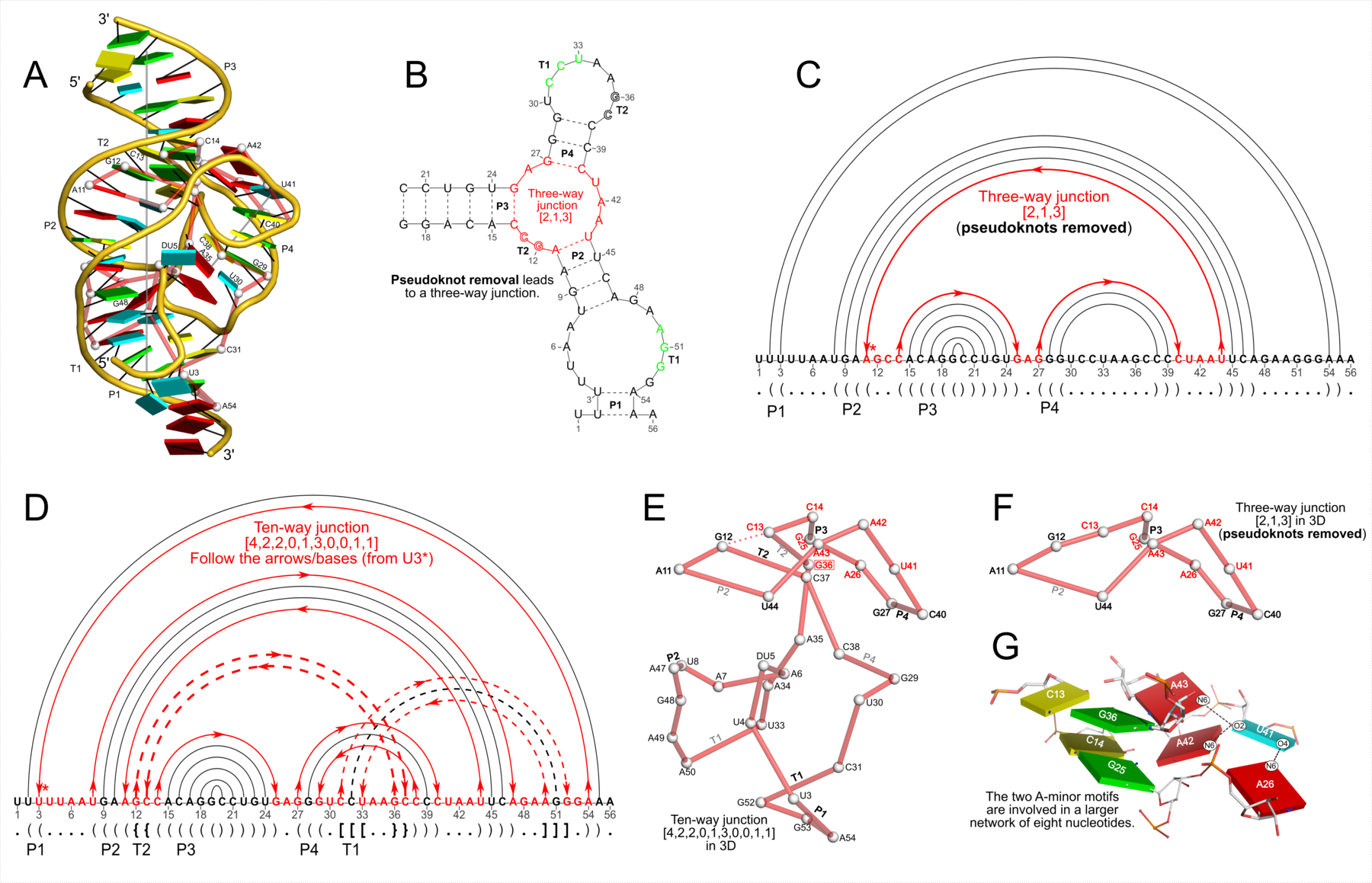
Quote
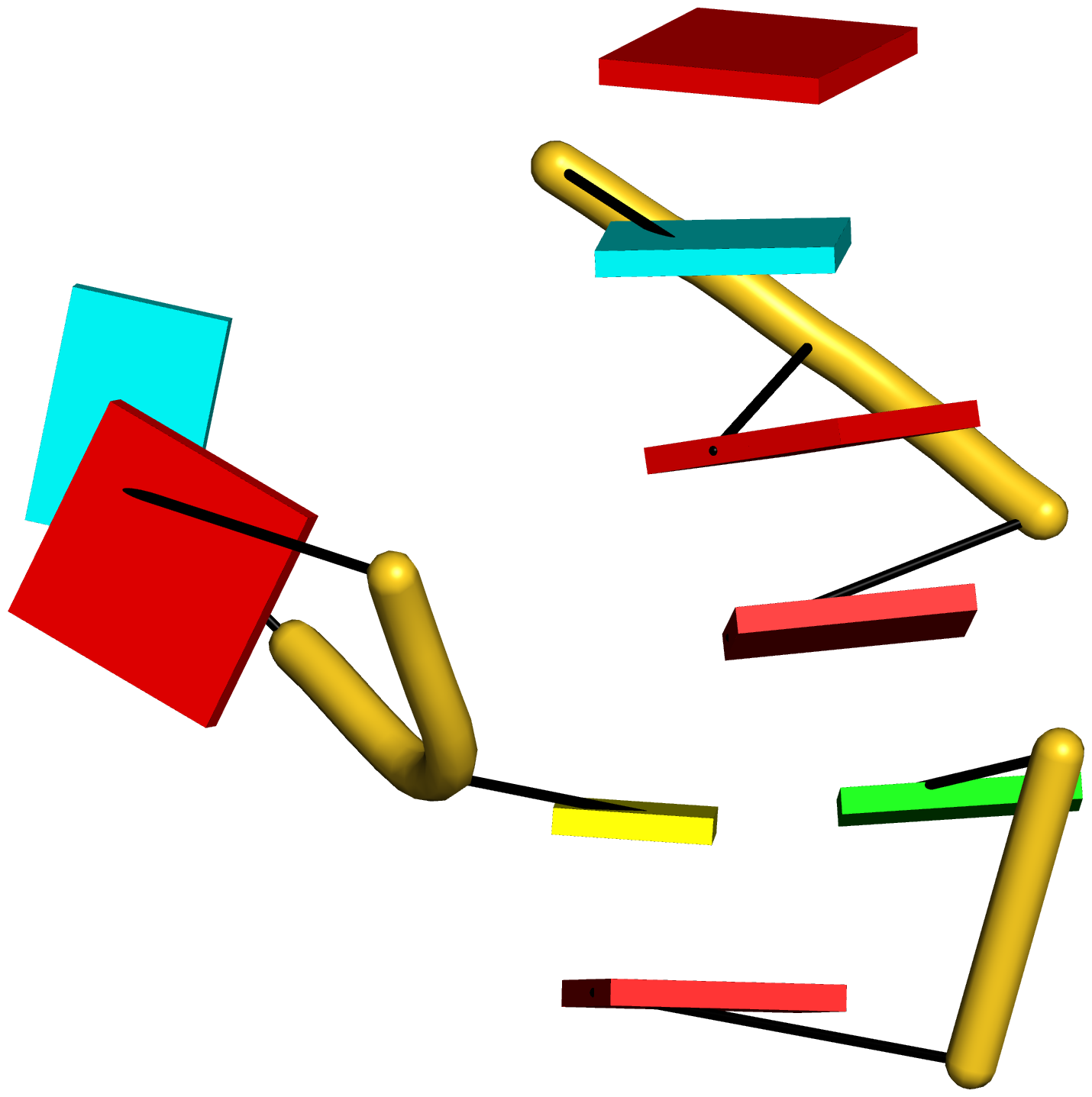
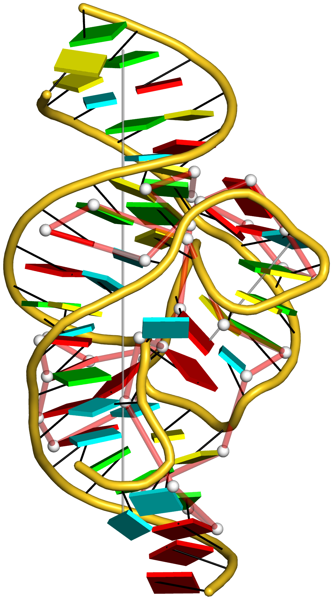
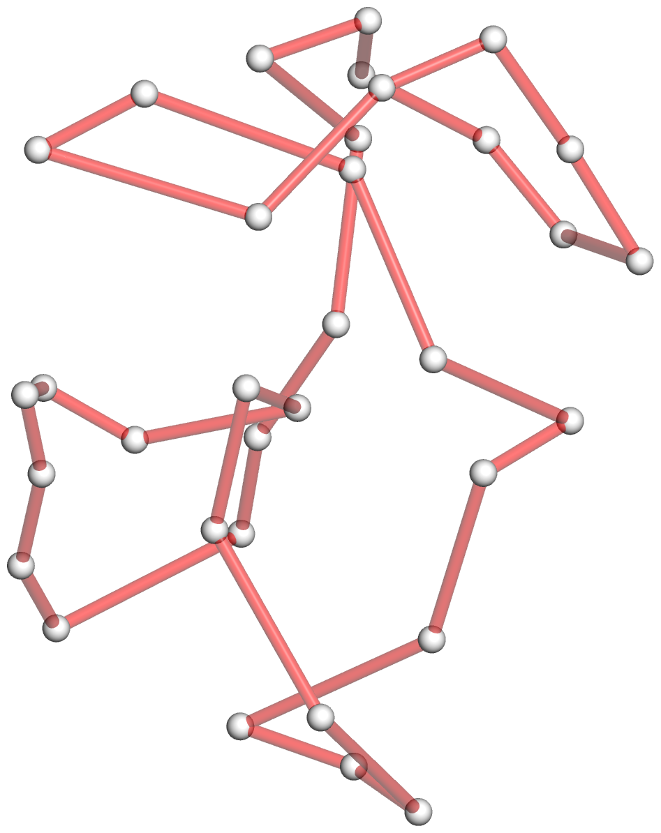
Figure 4: DSSR discloses complexity in the folding of the env22 twister ribozyme not apparent in the two-armed tertiary structure (chain A, PDB id: 4rge (43)). (A) The software automatically detects the long helical arm with five coaxially stacked stems and the short single-stemmed arm of the molecule. Failing to account for the pseudoknots within the structure leads to a characterization of the molecule very different from its real organization. When pseudoknots are omitted, the RNA appears to form a simplified [2,1,3] three-way junction as shown in both planar (B) and linear (C) secondary structure diagrams. In reality, the DSSR-derived dot-bracket notation points to a double-pseudoknotted structure (D) with two types of brackets distinguishing the pseudoknotted pairs (matched [] and {}), and uncovers a novel [4,2,2,0,1,3,0,0,1,1] ten-way junction loop (D,E). The junction, which can be traced by following the arrows along the red arcs and bases (starting from U3, marked with *) in D, contains both ends of four of the six stems and follows a supercoiled pathway in 3D (Supplementary Figure S5). In contrast, without consideration of pseudoknots (F), the junction forms a simple relaxed circle (Supplementary Figure S5). DSSR also detects three previously ignored base pairs that help to anchor the consecutive A-minor motifs reported in the literature (43) (G). U41 pairs with A42 and A43 through bifurcated hydrogen bonding, as well as with A26 (Supplementary Figure S4C,D). Moreover, U41 and A42 constitute a UpA dinucleotide platform, and in combination with G25 and A26, create a unique network of eight interacting nucleotides (G). All eight nucleotides are involved in the ten-way junction loop (labeled red in (E)).
Here is the tarball (fig4-twister-ribozyme-4rge.tar.gz) with the script and all related data files.
The content of the full script (named tasks) is shown below. Please see also notes for "Figure 2 -- analysis of the yeast phenylalanine tRNA (1ehz)".
Code: Bash
- # Step #1 -- reorient the twister ribozyme vertically
- pdb_frag A 1:56 4rge.pdb 4rge-A.pdb
- x3dna-dssr -i=4rge-A.pdb -o=4rge-A.out --more --prefix=4rge-A
- # To get the result illustrated in panel D, load '4rge-A-2ndstrs.ct'
- # or '4rge-A-2ndstrs.dbn' into VARNA to draw the linear secondary
- # structure diagram, exported as .svg for annotation in Inkscape.
- # Extract the two helical axes from 4rge-A.out to file: 4rge-A.rot1
- # then reorient the structure vertically: 4rge-A.rot2
- rotate_mol -t=4rge-A.rot1 4rge-A.pdb 4rge-A-rot1.pdb
- rotate_mol -r=4rge-A.rot2 4rge-A-rot1.pdb 4rge-A-ok.pdb
- # Step #2 -- get the cartoon-block representation with the two
- # ls-fitted helical axes.
- x3dna-dssr -i=4rge-A-ok.pdb --helical-axis -o=temp
- \mv dssr-helicalAxes.pdb 4rge-A-ok-helices.pdb
- x3dna-dssr -i=4rge-A-ok.pdb --block-file -o=4rge-A-ok-blocks.r3d
- # Step #3 -- simplified representation of the [4,2,2,0,1,3,0,0,1,1]
- # 10-way junction in 3D -- panel E
- # note the '--raw-xyz' option: it keeps the original coordinates
- x3dna-dssr -i=4rge-A-ok.pdb --raw-xyz --simple-junction -o=temp
- \mv dssr-simplifiedJcts.pdb 4rge-A-ok-jct.pdb
- # see file: 4rge-A-ok-jct.pml
- pymol -qkc 4rge-A-ok-jct.pml
- convert -trim +repage -border 10 -bordercolor white 4rge-A-ok-jct-pymol.png 4rge-A-ok-jct.png
- # see file: 4rge-A-ok-full.pml (cartoon-block with the schematic
- # junction overlaid) -- panel A
- pymol -qkc 4rge-A-ok-full.pml
- convert -trim +repage -border 10 -bordercolor white 4rge-A-ok-full-pymol.png 4rge-A-ok-full.png
- # Step #4 -- remove pseudoknots to get a fully nested structure. It now
- # has only a [2,1,3] 3-way junction -- panels B, C, and F
- \cp 4rge-A-ok.pdb 4rge-nested.pdb
- x3dna-dssr -i=4rge-nested.pdb --nested --raw-xyz --simple-junction --prefix=4rge-nested -o=4rge-nested.out
- # The planar (panel B) and linear (panel C) secondary structure
- # diagrams are produced by loading '4rge-nested-2ndstrs.ct' or
- # '4rge-nested-2ndstrs.dbn' into VARNA, exported as .svg, and
- # annotated with Inkscape.
- # see file: 4rge-nested-jct.pml -- panel F
- pymol -qkc 4rge-nested-jct.pml
- convert -trim +repage -border 10 -bordercolor white 4rge-nested-jct-pymol.png 4rge-nested-jct.png
- # Step #5 -- bifurcated U-A pairs in a network of 8 nucleotides
- pdb_frag A 13:14 A 25:26 A 36 A 41:43 4rge-A-ok.pdb 4rge-bifurcated.pdb
- x3dna-dssr -i=4rge-bifurcated.pdb --block-file -o=4rge-bifurcated.r3d
- # see file: 4rge-bifurcated.pml -- panel G
- pymol -qkc 4rge-bifurcated.pml
- convert -trim +repage -border 10 -bordercolor white 4rge-bifurcated-pymol.png 4rge-bifurcated.png
Here are the images generated from the above script:
68
DSSR-NAR paper / Figure 3 -- analysis of the tRNA mimic (4p5j)
« on: July 08, 2015, 08:38:47 pm »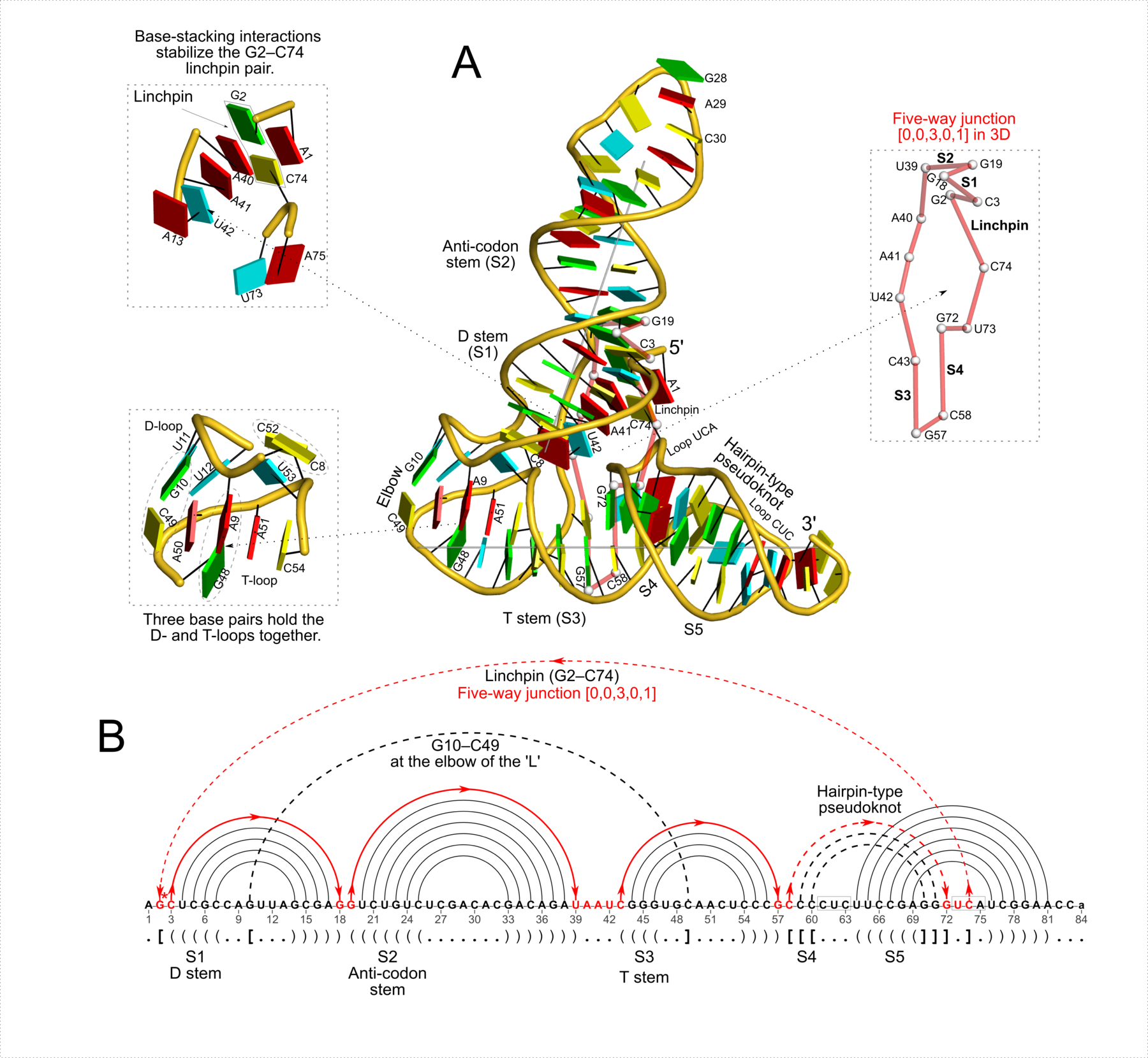
Quote
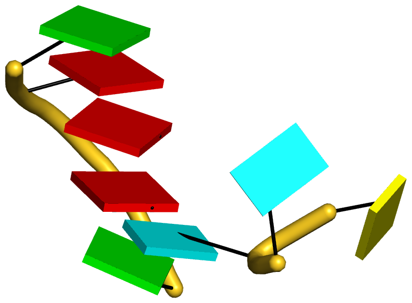
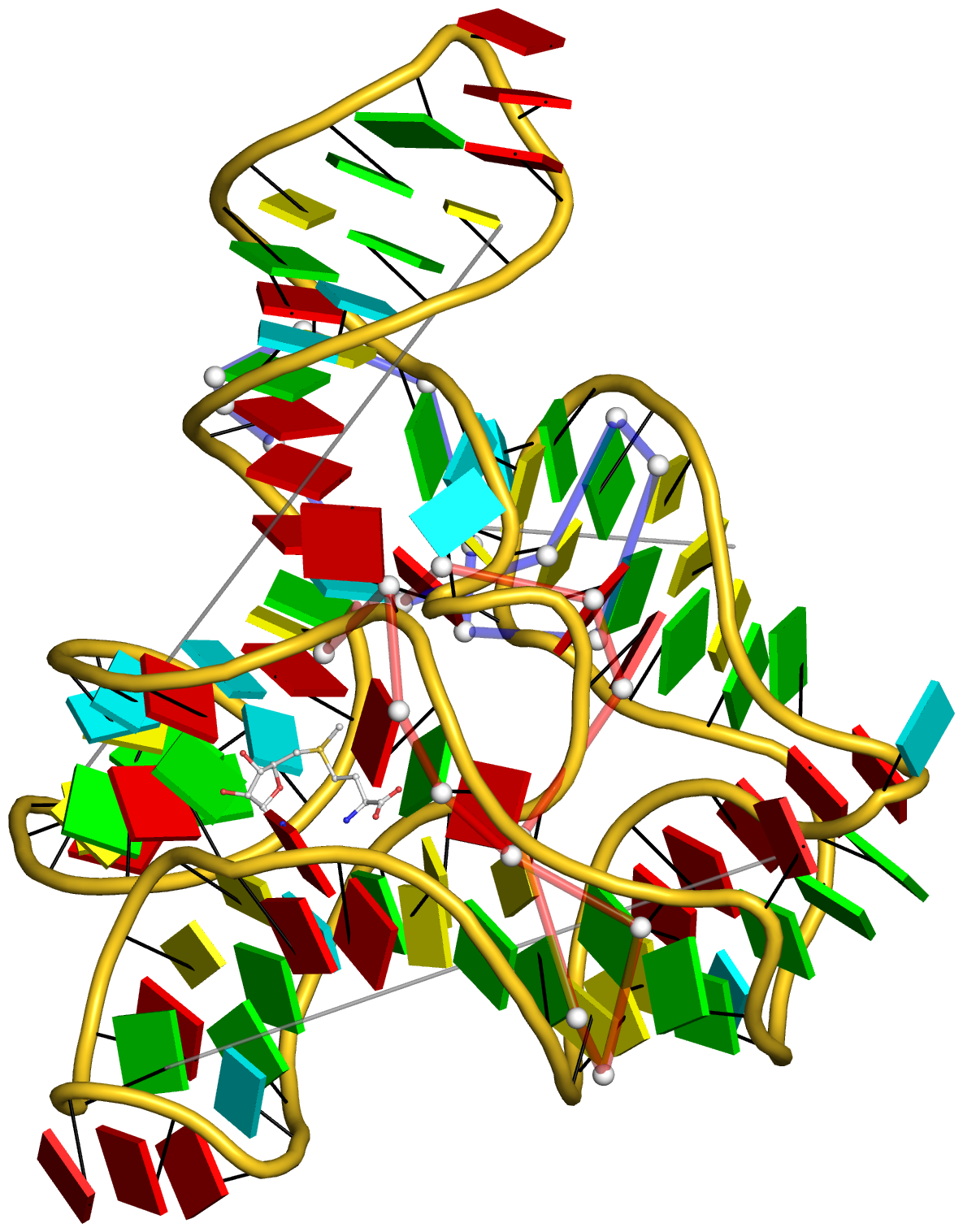
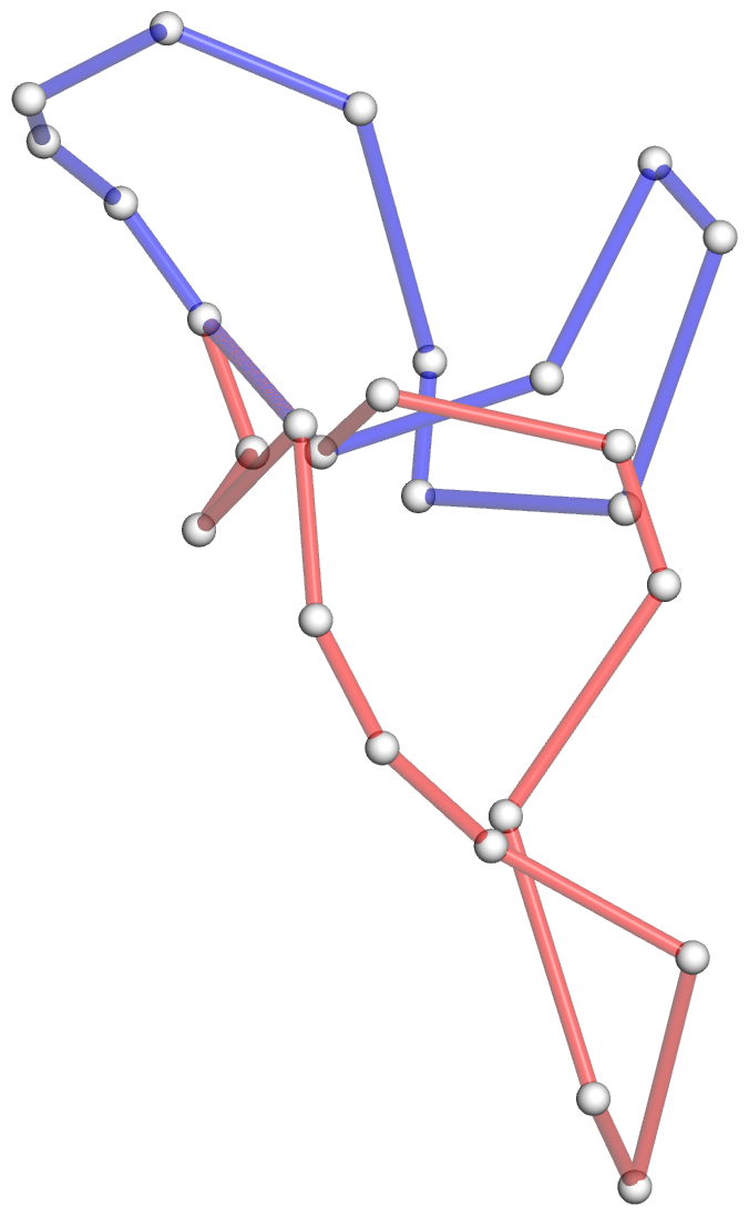
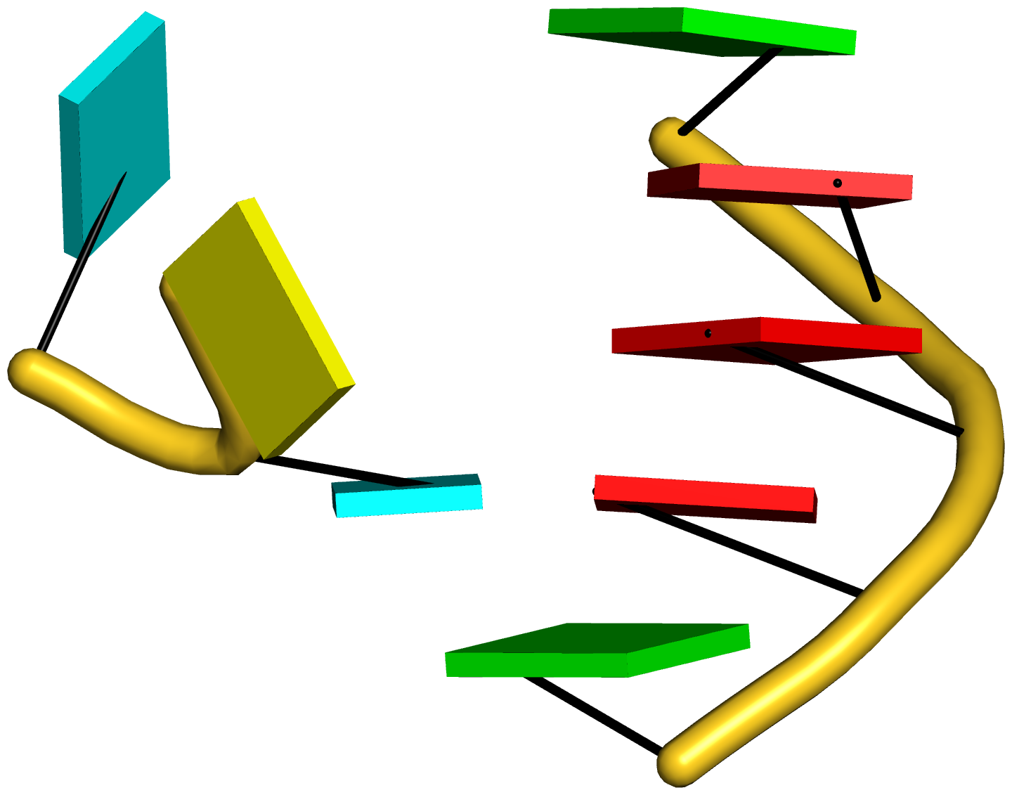
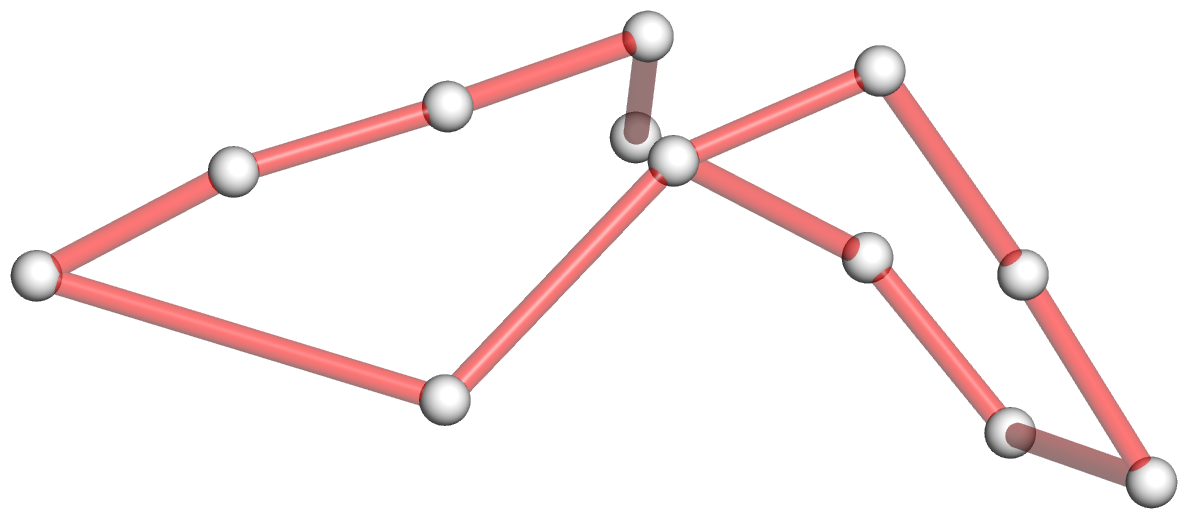
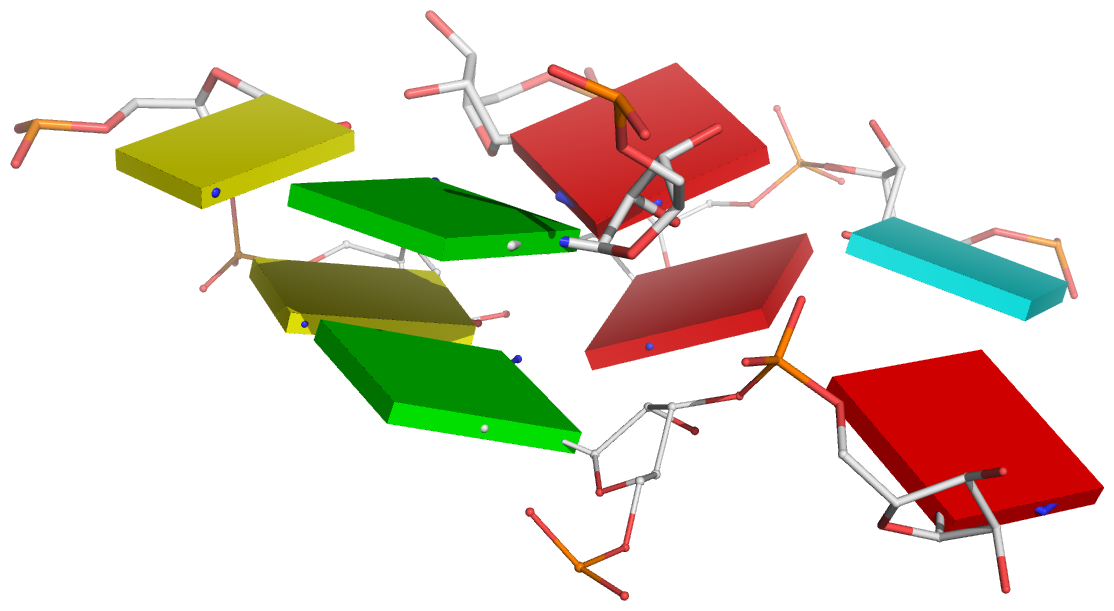
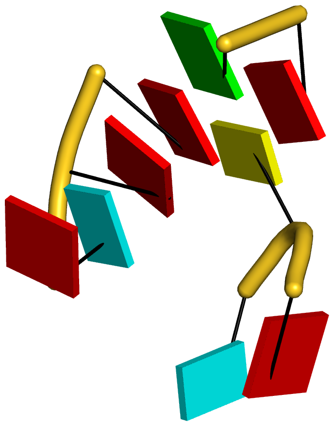
Figure 3: DSSR reveals the striking global similarity and distinct local variations between the tRNA mimic from turnip yellow mosaic virus (PDB id: 4p5j (34)) and yeast tRNAPhe. (A) The viral tRNA mimic assumes an overall L-shaped tertiary structure (center) composed of two helices (gray lines). DSSR uncovers a [0,0,3,0,1] five-way junction loop (right) enabled by the hairpin-type pseudoknot at the 3′-end of the molecule and the G2–C74 linchpin pair. This critical linchpin is unique to the tRNA mimic, where it is stabilized by extensive base-stacking interactions (upper-left). The lower-left inset emphasizes the intricate interactions between the D- and T-loops in the mimic, including the three base pairs (within dashed ellipses) and the unique base triplet at the elbow (Supplementary Figure S3A). (B) The linear secondary structure diagram generated with the DSSR-derived dot-bracket notation shows the sequential location of the bases comprising the linchpin pair, the five-way junction loop (red), the G10–C49 pair at the elbow, and the hairpin-type pseudoknot. Note that the dashed arcs connecting the so-called first-order pseudoknotted pairs (indicated by matched []) do not cross each other along the linear sequence. The numbering of residues used here follows that in the PDB file, which is offset by two nucleotides from that given in the original publication (e.g., the G2–C74 linchpin is termed G4–C76 there).
Here is the tarball (fig3-tRNA-mimic-4p5j.tar.gz) with the script and all related data files.
The content of the full script (named tasks) is shown below. Please see also notes for "Figure 2 -- analysis of the yeast phenylalanine tRNA (1ehz)".
Code: Bash
- # Step #1 -- reorient viral tRNA mimic into the classic "L" shape
- x3dna-dssr -i=4p5j.pdb -o=4p5j.out --more --prefix=4p5j
- # To get the result illustrated in panel B, load '4p5j-2ndstrs.ct' or
- # '4p5j-2ndstrs.dbn' into VARNA to draw the linear secondary structure
- # diagram, which is exported as .svg for annotation in Inkscape.
- pdb_frag A 1:84 4p5j.pdb 4p5j-nts.pdb
- # extract the two helical axes from 4p5j.out to file: 4p5j.rot1
- # then reorient the structure into the "L" shape: 4p5j.rot2
- rotate_mol -t=4p5j.rot1 4p5j-nts.pdb 4p5j-rot1.pdb
- rotate_mol -r=4p5j.rot2 4p5j-rot1.pdb 4p5j-ok.pdb
- # Step #2 -- get the cartoon-block representation with the two
- # ls-fitted helical axes.
- x3dna-dssr -i=4p5j-ok.pdb --helical-axis -o=temp
- \mv dssr-helicalAxes.pdb 4p5j-ok-helices.pdb
- x3dna-dssr -i=4p5j-ok.pdb --block-file -o=4p5j-ok-blocks.r3d
- # Step #3 -- simplified representation of the [0,0,3,0,1] 5-way junction in 3D
- # -- note the --raw-xyz option: it keeps the original coordinates
- x3dna-dssr -i=4p5j-ok.pdb --raw-xyz --simple-junction -o=temp
- \mv dssr-simplifiedJcts.pdb 4p5j-ok-jct.pdb
- # see file: 4p5j-ok-jct.pml
- pymol -qkc 4p5j-ok-jct.pml
- convert -trim +repage -border 10 -bordercolor white 4p5j-ok-jct-pymol.png 4p5j-ok-jct.png
- # see file: 4p5j-ok-full.pml (cartoon-block with the schematic junction overlaid)
- pymol -qkc 4p5j-ok-full.pml
- convert -trim +repage -border 10 -bordercolor white 4p5j-ok-full-pymol.png 4p5j-ok-full.png
- # Step #4 -- get the linchpin interactions
- pdb_frag A 1:2 A 40:42 A 13 A 73:75 4p5j-ok.pdb 4p5j-ok-linchpin.pdb
- x3dna-dssr -i=4p5j-ok-linchpin.pdb --block-file -o=4p5j-ok-linchpin-blocks.r3d
- pymol -qkc 4p5j-ok-linchpin.pml
- convert -trim +repage -border 10 -bordercolor white 4p5j-ok-linchpin-pymol.png 4p5j-ok-linchpin.png
- # Step #5 -- get the kissing loop interactions
- pdb_frag A 8:12 A 48:54 4p5j-ok.pdb 4p5j-ok-loops.pdb
- x3dna-dssr -i=4p5j-ok-loops.pdb --block-file -o=4p5j-ok-loops-blocks.r3d
- pymol -qkc 4p5j-ok-loops.pml
- convert -trim +repage -border 10 -bordercolor white 4p5j-ok-loops-pymol.png 4p5j-ok-loops.png
Here are the images generated from the above script:
69
DSSR-NAR paper / Figure 1 -- summary of methods to identify nucleic acid structural components
« on: July 08, 2015, 08:35:14 pm »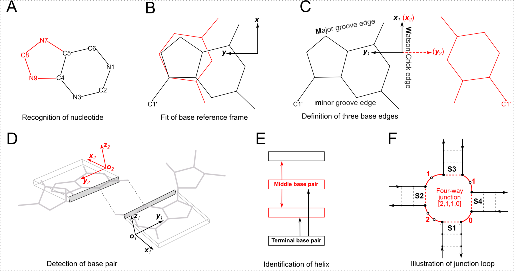
Quote
Figure 1: Summary of steps used to identify nucleic acid structural components. (A) Nucleotides are recognized using standard atom names and base planarity. A base is taken as a pyrimidine (six-membered ring) unless it possesses one of three purine atoms (red). (B) Bases are assigned a standard reference frame independent of sequence: purines and pyrimidines (red) are symmetrically placed with respect to the sugar. (C) The standard base frame is derived from an idealized Watson-Crick base pair, where the x1, y1-axes of the sequence base align with the x2-, y2-axes of its complement (red) and define three base edges (Watson-Crick, minor groove, Major groove). (D) Base pairs are identified from the distance and coplanarity of base rings (highlighted by rectangular blocks with embedded reference frames and shaded minor-groove edges) and the occurrence of at least one hydrogen bond (dashed lines). (E) Helices are defined by base-stacking interactions. Whereas the two nearest neighbors of a terminal pair (black) lie on one side of the pair, those of a middle pair (red) lie on opposite sides. (F) Closed loops are delineated by the ends of stems and specified by the lengths of consecutive connecting loop segments. Here, the four-way junction (S1 to S4) is denoted [2,1,1,0] in terms of the loop nucleotides (white circles) running clockwise from S1 to S4. Arrows point from the 5′ to 3′ direction along each strand and dashed lines represent stem pairs.
Note:
- This figure illustrates key algorithms implemented in DSSR for the analysis of nucleic acid structures. Many other features, such as the identification of pseudoknots and various motifs, are not included here for simplicity. The figure is composed using InkScape, going through numerous iterations and taking great attention to details.
- For identifying nucleotides (A), the nine ring atoms of guanine is used. Expressed in the standard base reference frame (see file 'Atomic_G.pdb' distributed with 3DNA), the atomic coordinates of the nine atoms in PDB format are as shown below. A nucleotide must have at least three properly labeled ring atoms, and the least-squares fitting (rmsd) between matched atom-pairs must be less than a cutoff (0.28 Å by default). Note that using adenine as the reference would have no impact on the result, as the base rings between G and A can be nearly perfectly aligned.
Code: [Select]
ATOM      2  N9    G A   1      -1.289   4.551   0.000
ATOM      3  C8    G A   1       0.023   4.962   0.000
ATOM      4  N7    G A   1       0.870   3.969   0.000
ATOM      5  C5    G A   1       0.071   2.833   0.000
ATOM      6  C6    G A   1       0.424   1.460   0.000
ATOM      8  N1    G A   1      -0.700   0.641   0.000
ATOM      9  C2    G A   1      -1.999   1.087   0.000
ATOM     11  N3    G A   1      -2.342   2.364   0.001
ATOM 12 C4 G A 1 -1.265 3.177 0.000- The standard base reference frame has unique features (B). It is symmetric to purines/pyrimidines and independent of base sequence. The standard frame also enjoys simple geometric meaning with its three axes. Overall, the frame fits perfectly for the analysis of RNA structures and is superior to other ad hoc frames seen in literature.
- DSSR introduces three edges that are strictly base centered (C): the minor-groove edge, the Major-groove edge, and the Watson-Crick edge. The major-groove edge corresponds to the Hoogsteen/C-H edge in the Leontis-Westhof (LW) notation. The minor-groove edge correlates with the LW sugar edge only when the base is in the anti conformation, and the sugar is in C3′-endo conformation in RNA. See the User Manual for details.
- When the standard reference frames are attached to the planar base rings (D), the geometric-based definition of base pairs (first introduced in 3DNA over 15 years ago) is immediately obvious. Moreover, the algorithm applies to canonical as well as noncanonical base pairs, including those with modified nucleotides, in any tautomeric or protonation state.
- DSSR's definition of helices and stems is illustrated in (E). It distinguishes a stem of covalently connected canonical pairs from a helix of stacked pairs of arbitrary type/linkage. This differentiation leads naturally to a definition of coaxial stacking, another widely used concept. Moreover, the same algorithm also applies to the identification of continuous base stacks.
- In DSSR, a loop forms a 'closed' circle (F) with any two sequential nucleotides connected either by a phosphodiester bond or a canonical base pair, and is specified by the lengths of consecutive bridging-nucleotide segments.
70
DSSR-NAR paper / Figure 2 -- analysis of the yeast phenylalanine tRNA (1ehz)
« on: July 08, 2015, 08:33:05 pm »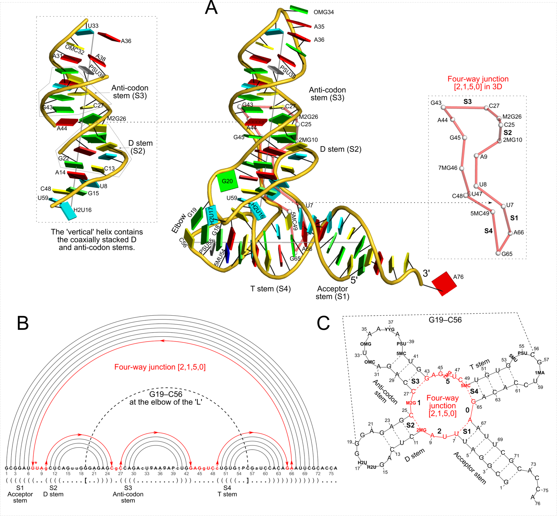
Quote
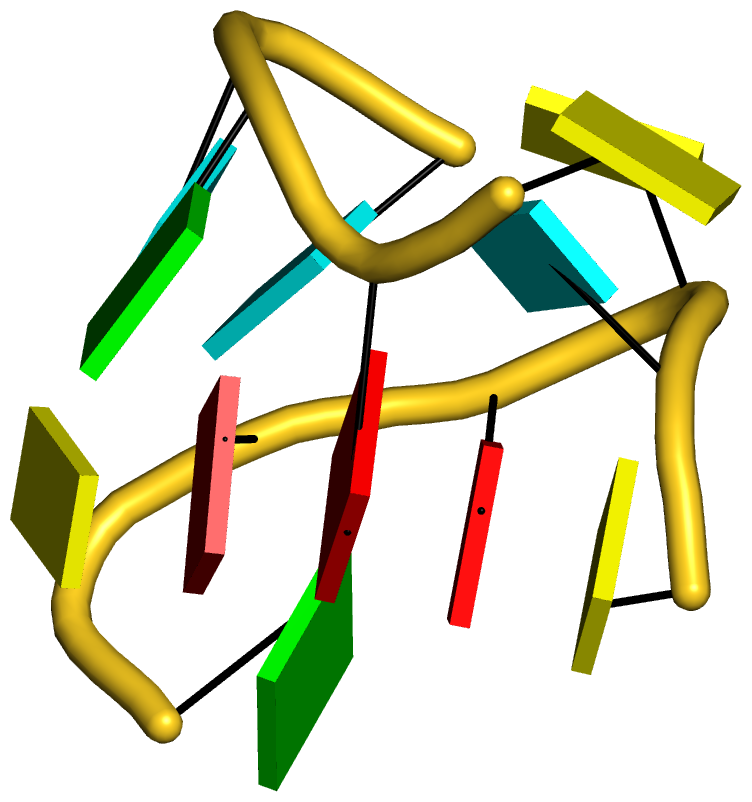
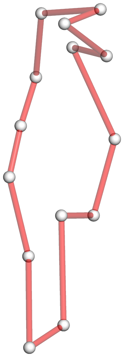
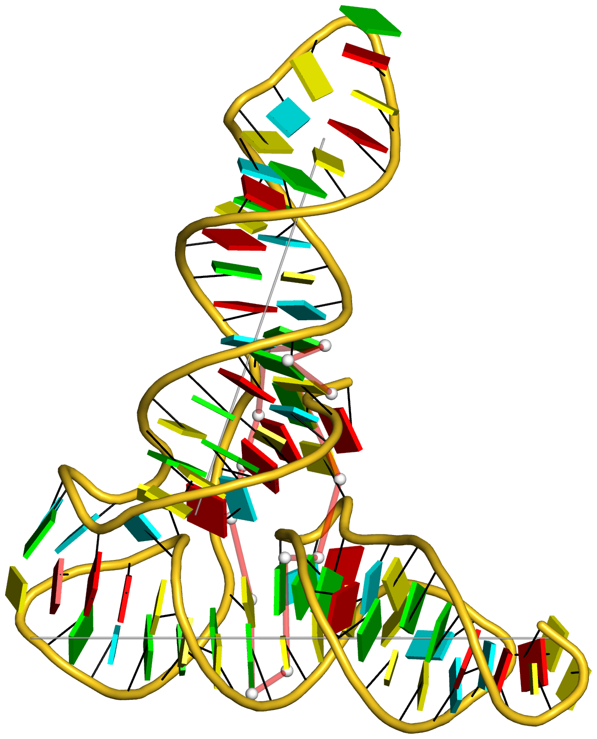
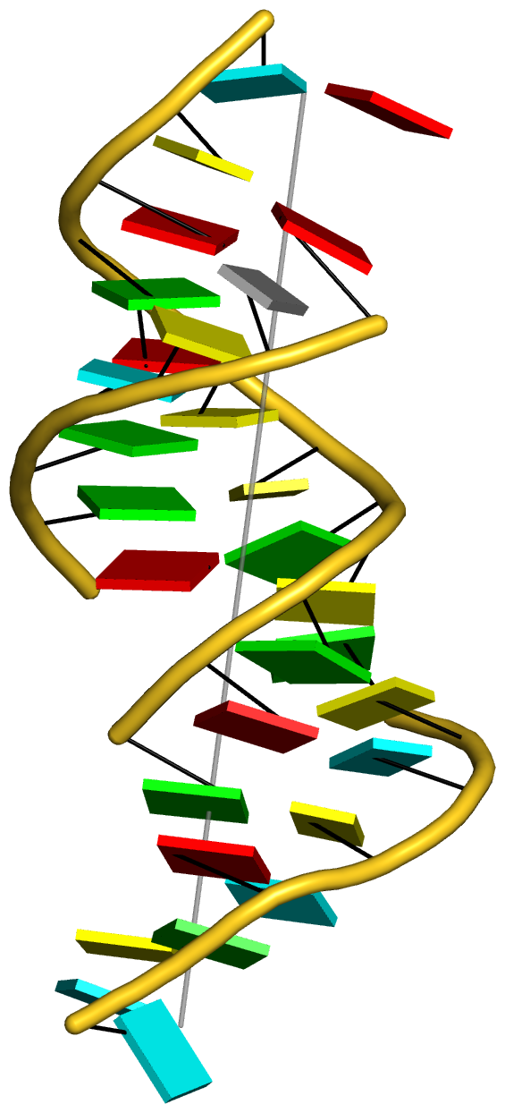
Figure 2: DSSR captures well-known features and provides a new perspective on the classic yeast tRNAPhe structure (PDB id: 1ehz (46)). (A) The software automatically detects the four stems and the two helices that form the L-shaped molecule, depicted here in cartoon-block representation (center). Whereas the helices may include all types of base pairs and backbone breaks, the stems comprise only canonical pairs with continuous backbones. Note the coaxial stacking of the D and anti-codon stems and the noncanonical features of the composite helix (represented by a gray line, left). The red ‘circle’, overlaid on the central image and detailed to the right, reveals the 3D pathway along the [2,1,5,0] four-way junction loop. (B) The dot-bracket notation derived by DSSR serves as input for the depicted linear (arc) representation of secondary structure. The bases comprising the four-way junction loop (red) run in sequential order from U7 (*) following the arrows to the right and returning along the outer A66→U7 arc. The pseudoknotted G19–C56 pair (with matched []) is noted by the dashed arc. (C) Both the four-way junction (red) and the three hairpin loops follow ‘circular’ routes within the traditional cloverleaf representation of tRNA. Here the 14 modified nucleotides are represented by three-letter codes. The 3D images were created using PyMOL (A-red; C-yellow; G-green; T-blue; U-cyan; pseudouridine P-gray), the 2D diagrams using VARNA, and the annotations using Inkscape.
Here is the tarball (fig2-tRNA-1ehz.tar.gz) containing all the scripts and data files.
It takes many steps and great attention to details to generate the above figure, even though the basic idea is quite simple. The following script (in file 'tasks') takes advantage of 3DNA, PyMOL, VARNA, ImageMagick, Inkscape and some previously undocumented DSSR options. It is not the raw script originally used to create Figure 2 of the DSSR-NAR paper. For easy followup, the script has been made more self-contained, at the expense of apparent repetition of commands and PyMOL settings in various .pml files.
For understanding of the script, detailed notes are provided below for each major step. The 3D images in .png format and secondary structure diagrams in .svg format are combined and annotated using Inkscape. Great care has been taken to ensure the accuracy of details and quality of the figure. By and large, Figures 3-6 and Supplementary Figures 1-9 follow the same convention.
Code: Bash
- # Step #1 -- reorient tRNA into the classic "L" shape
- x3dna-dssr -i=1ehz.pdb -o=1ehz.out --more --prefix=1ehz
- pdb_frag A 1:76 1ehz.pdb 1ehz-nts.pdb
- # extract the two helical axes from 1ehz.out to file: 1ehz.rot1
- # then reorient the structure into the "L" shape: 1ehz.rot2
- rotate_mol -t=1ehz.rot1 1ehz-nts.pdb 1ehz-rot1.pdb
- rotate_mol -r=1ehz.rot2 1ehz-rot1.pdb 1ehz-ok.pdb
- # Step #2 -- get the cartoon-block representation with the two
- # ls-fitted helical axes.
- x3dna-dssr -i=1ehz-ok.pdb --helical-axis -o=temp
- \mv dssr-helicalAxes.pdb 1ehz-ok-helices.pdb
- x3dna-dssr -i=1ehz-ok.pdb --block-file -o=1ehz-ok-blocks.r3d
- # Step #3 -- simplified representation of the [2,1,5,0] 4-way junction in 3D
- # -- note the --raw-xyz option: it keeps the original coordinates
- x3dna-dssr -i=1ehz-ok.pdb --raw-xyz --simple-junction -o=temp
- \mv dssr-simplifiedJcts.pdb 1ehz-ok-jct.pdb
- # see file: 1ehz-ok-jct.pml
- pymol -qkc 1ehz-ok-jct.pml
- convert -trim +repage -border 10 -bordercolor white 1ehz-ok-jct-pymol.png 1ehz-ok-jct.png
- # see file: 1ehz-ok-full.pml (cartoon-block with the schematic junction overlaid)
- pymol -qkc 1ehz-ok-full.pml
- convert -trim +repage -border 10 -bordercolor white 1ehz-ok-full-pymol.png 1ehz-ok-full.png
- # Step #4 -- illustration of 'vertical' helix of the "L", composed of
- # anti-codon and D stems, coaxially stacked around M2G26-A44
- x3dna-dssr -i=1ehz-ok.pdb --raw-xyz -o=temp
- ex_str -2 dssr-helices.pdb 1ehz-ok-h2.pdb
- x3dna-dssr -i=1ehz-ok-h2.pdb --helical-axis -o=temp
- \mv dssr-helicalAxes.pdb 1ehz-ok-h2-helices.pdb
- x3dna-dssr -i=1ehz-ok-h2.pdb --block-file -o=1ehz-ok-h2-blocks.r3d
- # see file: 1ehz-ok-h2.pml
- pymol -qkc 1ehz-ok-h2.pml
- convert -trim +repage -border 10 -bordercolor white 1ehz-ok-h2-pymol.png 1ehz-ok-h2.png
Step #1: reorient the raw tRNA PDB structure (1ehz) into the classic "L" shape. The helix containing the acceptor/T stems is put "horizontal", and the one with D/anti-codon stems "vertical".
- The DSSR --prefix option gives rise to three files 1ehz-2ndstrs.ct, 1ehz-2ndstrs.dbn and 1ehz-2ndstrs.bpseq for the representations of the secondary structure. Overall, the .ct format is more informative, and .dbn most compact. Any of the three files can be loaded directly into VARNA for the visualization of the secondary structure. There are many settings one can play with in VARNA. In Panel B and C, I used the simple "Line" BP style, set number period to 3, clicked "Toggle draw bases" etc. In VARNA, Panel B is in the so-called "Linear" style, and Panel C in "Radiate" style. The VARNA secondary structure diagrams are exported into .svg format for further annotation in Inkscape.
- The first DSSR run (line no.2) specifies the --more option to output detailed output of the two helical axes in file 1ehz.out
  helix#1[2] bps=15
      strand-1 5'-GCGGAUUcUGUGtPC-3'
       bp-type    ||||||||||||..|
      strand-2 3'-CGCUUAAGACACaGG-5'
      helix-form  AA....xAAAAxx.
    helical-rise:   3.00(0.90) *
    helical-radius: 8.88(1.77) *
    helical-axis:    0.617     0.739    -0.269 *

  helix#2[2] bps=15
      strand-1 5'-AAPcUGGAgCUCAGu-3'
       bp-type    ...||||.||||...
      strand-2 3'-UcAGACCgCGAGUCU-5'
      helix-form  x..AAAAxAA.xxx
    helical-rise:   3.07(1.12) *
    helical-radius: 8.89(2.35) *
helical-axis: 0.071 0.444 0.893 * - The pdb_frag utility program from 3DNA (in folder $X3DNA/perl_scripts) extracts all the 76 nucleotides on chain A of 1ehz.pdb to 1ehz-nts.pdb. The script is included here for completeness.
- The vectors of the two helical axes are collected into file 1ehz.rot1 to set the structure (using rotate_mol) into an orientation shown below. See also "Recipe no. 4: command-line script to illustrate the three helices in a four-way DNA-RNA junction" of the 2008 3DNA Nature Protocols paper.
     1  # x-, y-, z-axes row-rise
      0.000    0.000    0.000   # translation
      0.617    0.739   -0.269   # h1
      0.071    0.444    0.893   # h2
      0.000   0.000   1.000   # z: can be anything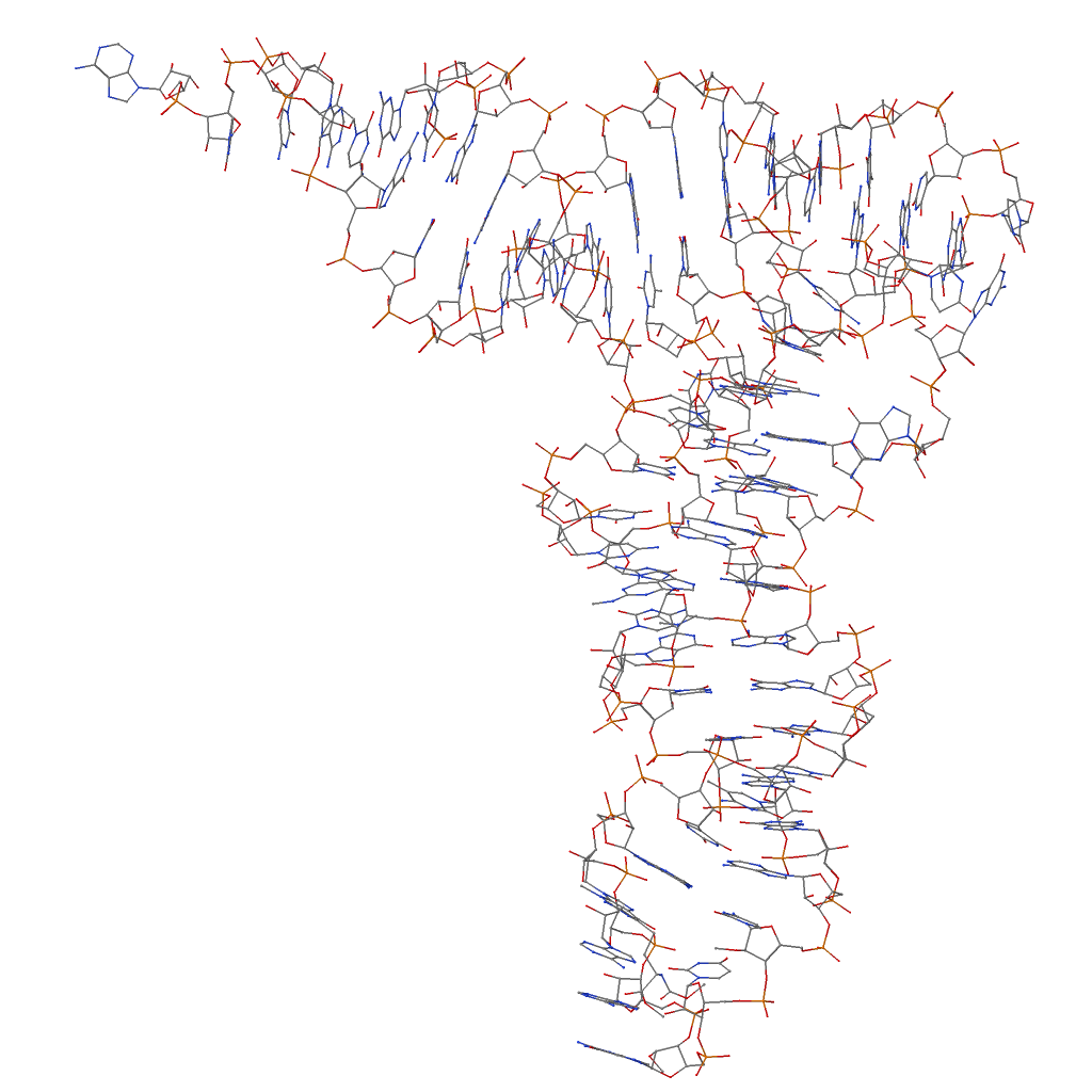
- The second run of rotate_mol put the tRNA (1ehz) into its final orientation (1ehz-ok.pdb). The content of 1ehz.rot2
is as below:by rotation y 180
The transformed PDB coordinate file 1ehz-ok.pdb is the starting point of all the following illustrations.
by rotation x 180
Step #2: -- get the cartoon-block representation with the two least-squares-fitted helical axes.
- The DSSR --helical-axis option generates the auxiliary file dssr-helicalAxes.pdb, which contains the two end points for each helix. The file is renamed 1ehz-ok-helices.pdb for easy reference, and has the following content:
REMARK-DSSR: helix#1
ATOM      1  P1    G A   1     -50.221 -58.766  28.361  1.00 99.85      H1   P
REMARK-DSSR: helix#1
ATOM      2  P2    C A  56     -92.115 -58.758  28.363  1.00 37.81      H1   P
REMARK-DSSR: helix#2
ATOM      3  P1    A A  36     -70.051  -7.424  32.844  1.00 81.67      H2   P
REMARK-DSSR: helix#2
HETATM    4  P2  H2U A  16     -75.673 -49.918  32.841  1.00 64.01      H2   P
CONECT    1    2
CONECT    2    1
CONECT    3    4
CONECT 4 3 - The DSSR --block-file option creates a file named "1ehz-ok-blocks.r3d" in Raster3D .r3d format, with bases in rectangular block representation. The .r3d file can not only be read by render of Raster3D, but also by PyMOL.
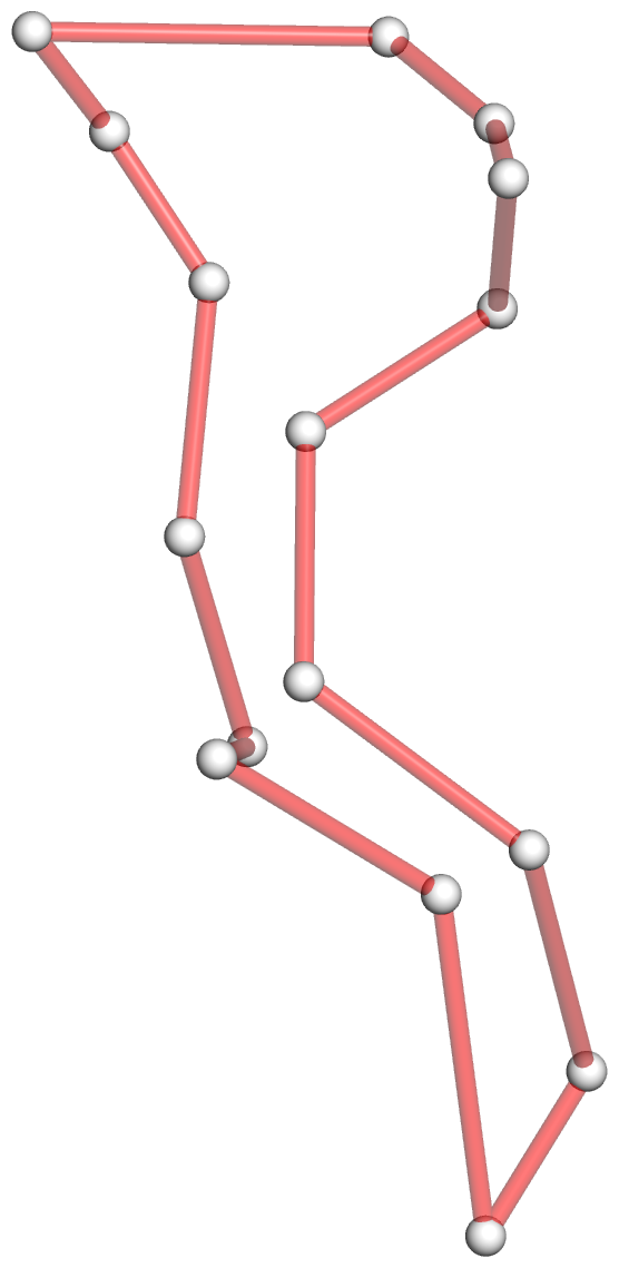
Step #3 -- simplified representation of the [2,1,5,0] 4-way junction in 3D
- The DSSR --raw-xyz option makes the auxiliary PDB files in the original coordinates instead of in certain new reference frames. For example, by default, the dssr-pairs.pdb file has each pair in the its own reference frame (top view) that enables easy comparison and visualization. Here, the --raw-xyz option is used to ensure a direct comparison of the 4-way junction loop in isolation vs that overlaid within the whole tRNA structure (1ehz-ok.pdb). The default junction file dssr-junctions.pdb is renamed 1ehz-ok-4wj.pdb for easy reference.
- The DSSR --simple-junction option produces another auxiliary file, named dssr-simplifiedJcts.pdb by default, and renamed 1ehz-ok-jct.pdb for easy reference. The file contains the atomic coordinates of C1′ atoms of the 4-way junction loop, with content shown below. Note that the nucleotides are in proper sequential order.
MODEL        1
REMARK    model=1  nts=16
REMARK    4-way junction: nts=16; [2,1,5,0]; linked by [#1,#2,#3,#4]
ATOM      1  C1'   U A   7     -65.936 -49.847  29.027  1.00 37.23           C
ATOM      2  C1'   U A   8     -72.670 -44.818  30.530  1.00 30.28           C
ATOM      3  C1'   A A   9     -72.606 -37.344  27.403  1.00 28.79           C
HETATM    4  C1' 2MG A  10     -66.888 -33.680  24.426  1.00 44.62           C
ATOM      5  C1'   C A  25     -66.556 -29.785  34.413  1.00 51.93           C
HETATM    6  C1' M2G A  26     -66.983 -28.143  29.356  1.00 46.92           C
ATOM      7  C1'   C A  27     -70.138 -25.556  25.591  1.00 48.68           C
ATOM      8  C1'   G A  43     -80.779 -25.396  27.582  1.00 46.94           C
ATOM      9  C1'   A A  44     -78.474 -28.381  24.234  1.00 54.14           C
ATOM     10  C1'   G A  45     -75.498 -32.895  24.403  1.00 45.24           C
HETATM   11  C1' 7MG A  46     -76.230 -40.483  24.555  1.00 39.69           C
ATOM     12  C1'   U A  47     -74.362 -46.762  19.557  1.00 50.55           C
ATOM     13  C1'   C A  48     -75.266 -47.135  28.377  1.00 27.98           C
HETATM   14  C1' 5MC A  49     -68.564 -51.174  23.872  1.00 33.10           C
ATOM     15  C1'   G A  65     -67.234 -61.378  20.695  1.00 42.23           C
ATOM     16  C1'   A A  66     -64.217 -56.459  21.032  1.00 40.50           C
CONECT    1   16    2
CONECT    2    1    3
CONECT    3    2    4
CONECT    4    3    5
CONECT    5    4    6
CONECT    6    5    7
CONECT    7    6    8
CONECT    8    7    9
CONECT    9    8   10
CONECT   10    9   11
CONECT   11   10   12
CONECT   12   11   13
CONECT   13   12   14
CONECT   14   13   15
CONECT   15   14   16
CONECT   16   15    1
ENDMDL - The 4-way junction in a simplified representation is ray-traced with PyMOL based on 1ehz-ok-jct.pml. The style of the 4-way junction is controlled by various PyMOL settings, as shown below.
load 1ehz-ok-jct.pdb, jct
The PyMOL options -qkc is used to generate file 1ehz-ok-jct-pymol.png from command line. Note the extra white space around the image (see below).
hide everything, jct
set sphere_color, white, jct
set sphere_scale, 0.36, jct
show spheres, jct
set stick_radius, 0.3, jct
set stick_color, red, jct
set stick_transparency, 0.46, jct
show sticks, jct
# -----------------------------------------
bg_color white
util.cbaw
set sphere_quality, 4
set stick_quality, 16
# PyMOL FAQ recommendations
set depth_cue, 0
set ray_trace_fog, 0
set ray_shadow, off
set orthoscopic, 1
set antialias, 1
# cannot be: zoom complete, 1
zoom complete=1
# -----------------------------------------
ray 1800
png 1ehz-ok-jct-pymol.png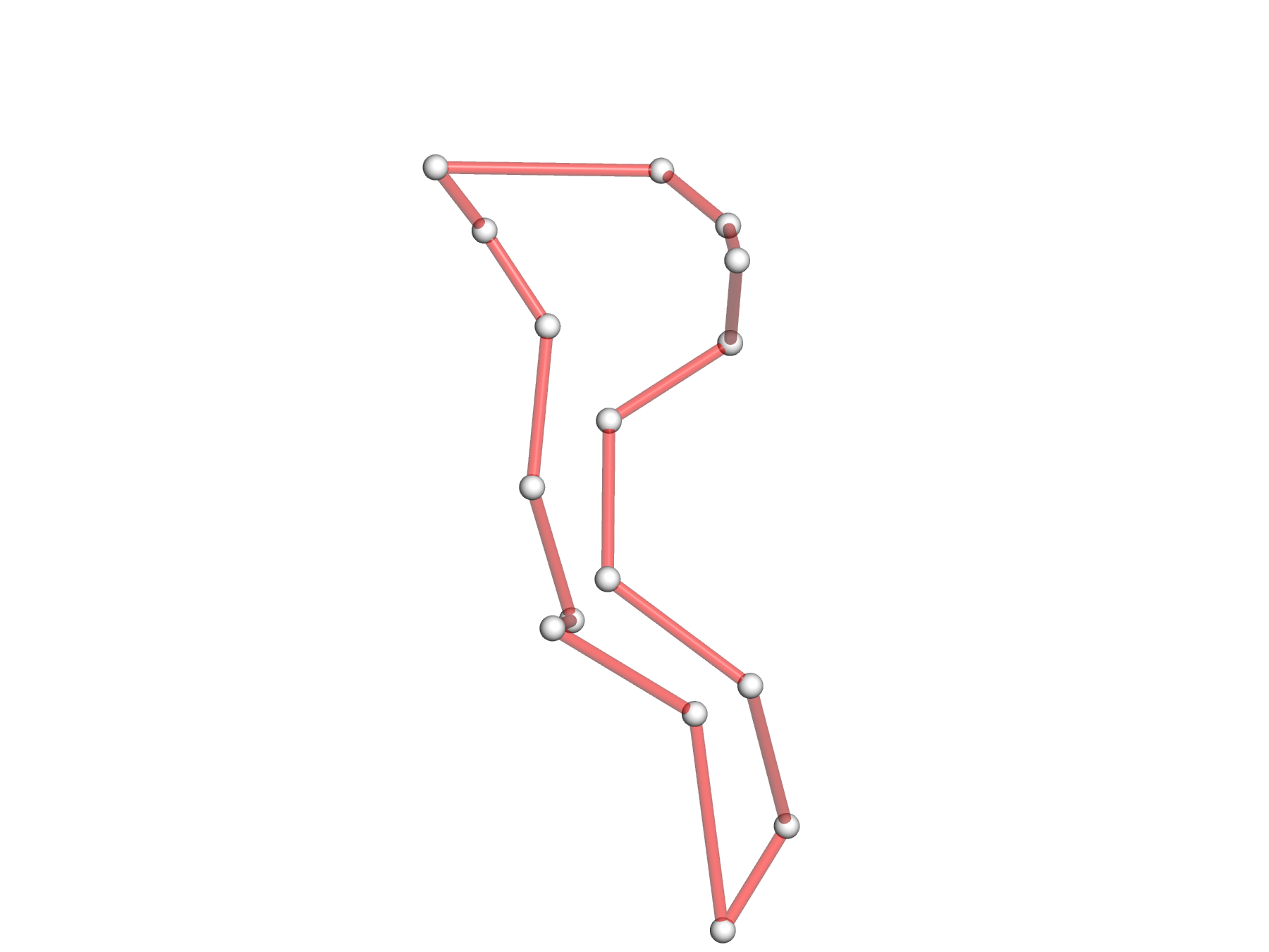
- The convert command from the popular ImageMagick package is employed simply to crop the extra white space around PyMOL-generated png image.
- The 1ehz-ok-full.pml PyMOL script combines all the components (backbone cartoon with ladder for bases, colored base rectangular blocks, gray helical axes, and the overlaid schematic 4-way junction loop) to generate the main part of panel A of the figure. See below:

Step #4 -- illustration of 'vertical' helix of the L-shaped tRNA
- Note the three options --raw-xyz, --helical-axis, and --block-file mentioned above.
- The PyMOL script file is 1ehz-ok-h2.pml, and the final generated image is shown below:
71
DSSR-NAR paper / Output of a sample DSSR run on yeast phenylalanine tRNA (1ehz)
« on: July 08, 2015, 12:41:25 pm »
This analysis is straightforward, and takes virtually no time. The command is shown in the output file as well:
For completeness, here is the original 1ehz.out file included in the Supplementary Data file of the DSSR paper.
Note the 14 modified nucleotides (shown below) auto-identified by DSSR:
For simplicity, the --more option is excluded from the sample DSSR run. Otherwise, neat listings would be distracted by additional auxiliary parameters. For example, the section listing base pairs (without specifying --more as in the above 1ehz.out file) is shown below:
More informative, but less intuitive. As noted in the User Manual, "There is more to DSSR than meets the eye. By connecting dots in RNA structural bioinformatics, the program makes many common tasks simple and advanced applications feasible."
Code: [Select]
x3dna-dssr -i=1ehz.pdb --u-turn --non-pair --po4 -o=1ehz.outFor completeness, here is the original 1ehz.out file included in the Supplementary Data file of the DSSR paper.
Code: [Select]
****************************************************************************
DSSR: an Integrated Software Tool for
Dissecting the Spatial Structure of RNA
v1.2.8-2015jun15 by xiangjun@x3dna.org
This program is being actively maintained and developed. As always,
I greatly appreciate your feedback! Please report all DSSR-related
issues on the 3DNA Forum (forum.x3dna.org). I strive to respond
*promptly* to *any questions* posted there.
****************************************************************************
Note: Each nucleotide is identified by model:chainId.name#, where the
'model:' portion is omitted if no model number is available (as
is often the case for x-ray crystal structures in the PDB). So a
common example would be B.A1689, meaning adenosine #1689 on
chain B. One-letter base names for modified nucleotides are put
in lower case (e.g., 'c' for 5MC). For further information about
the output notation, please refer to the DSSR User Manual.
Questions and suggestions are always welcome on the 3DNA Forum.
Command: x3dna-dssr -i=1ehz.pdb --u-turn --non-pair --po4 -o=1ehz.out
Date and time: Mon Jun 15 02:58:49 2015
File name: 1ehz.pdb
no. of DNA/RNA chains: 1 [A=76]
no. of nucleotides: 76
no. of atoms: 1821
no. of waters: 160
no. of metals: 9 [Mg=6,Mn=3]
****************************************************************************
List of 11 types of 14 modified nucleotides
nt count list
1 1MA-a 1 A.1MA58
2 2MG-g 1 A.2MG10
3 5MC-c 2 A.5MC40,A.5MC49
4 5MU-t 1 A.5MU54
5 7MG-g 1 A.7MG46
6 H2U-u 2 A.H2U16,A.H2U17
7 M2G-g 1 A.M2G26
8 OMC-c 1 A.OMC32
9 OMG-g 1 A.OMG34
10 PSU-P 2 A.PSU39,A.PSU55
11 YYG-g 1 A.YYG37
****************************************************************************
List of 34 base pairs
nt1 nt2 bp name Saenger LW DSSR
1 A.G1 A.C72 G-C WC 19-XIX cWW cW-W
2 A.C2 A.G71 C-G WC 19-XIX cWW cW-W
3 A.G3 A.C70 G-C WC 19-XIX cWW cW-W
4 A.G4 A.U69 G-U Wobble 28-XXVIII cWW cW-W
5 A.A5 A.U68 A-U WC 20-XX cWW cW-W
6 A.U6 A.A67 U-A WC 20-XX cWW cW-W
7 A.U7 A.A66 U-A WC 20-XX cWW cW-W
8 A.U8 A.A14 U-A rHoogsteen 24-XXIV tWH tW-M
9 A.U8 A.A21 U+A -- n/a tSW tm+W
10 A.A9 A.A23 A+A -- 02-II tHH tM+M
11 A.2MG10 A.C25 g-C WC 19-XIX cWW cW-W
12 A.2MG10 A.G45 g+G -- n/a cHS cM+m
13 A.C11 A.G24 C-G WC 19-XIX cWW cW-W
14 A.U12 A.A23 U-A WC 20-XX cWW cW-W
15 A.C13 A.G22 C-G WC 19-XIX cWW cW-W
16 A.G15 A.C48 G+C rWC 22-XXII tWW tW+W
17 A.H2U16 A.U59 u+U -- n/a tSW tm+W
18 A.G18 A.PSU55 G+P -- n/a tWS tW+m
19 A.G19 A.C56 G-C WC 19-XIX cWW cW-W
20 A.G22 A.7MG46 G-g -- 07-VII tHW tM-W
21 A.M2G26 A.A44 g-A Imino 08-VIII cWW cW-W
22 A.C27 A.G43 C-G WC 19-XIX cWW cW-W
23 A.C28 A.G42 C-G WC 19-XIX cWW cW-W
24 A.A29 A.U41 A-U WC 20-XX cWW cW-W
25 A.G30 A.5MC40 G-c WC 19-XIX cWW cW-W
26 A.A31 A.PSU39 A-P -- n/a cWW cW-W
27 A.OMC32 A.A38 c-A -- n/a c.W c.-W
28 A.U33 A.A36 U-A -- n/a tSH tm-M
29 A.5MC49 A.G65 c-G WC 19-XIX cWW cW-W
30 A.U50 A.A64 U-A WC 20-XX cWW cW-W
31 A.G51 A.C63 G-C WC 19-XIX cWW cW-W
32 A.U52 A.A62 U-A WC 20-XX cWW cW-W
33 A.G53 A.C61 G-C WC 19-XIX cWW cW-W
34 A.5MU54 A.1MA58 t-a rHoogsteen 24-XXIV tWH tW-M
****************************************************************************
List of 4 multiplets
1 nts=3 UAA A.U8,A.A14,A.A21
2 nts=3 AUA A.A9,A.U12,A.A23
3 nts=3 gCG A.2MG10,A.C25,A.G45
4 nts=3 CGg A.C13,A.G22,A.7MG46
****************************************************************************
List of 2 helices
Note: a helix is defined by base-stacking interactions, regardless of bp
type and backbone connectivity, and may contain more than one stem.
helix#number[stems-contained] bps=number-of-base-pairs in the helix
bp-type: '|' for a canonical WC/wobble pair, '.' otherwise
helix-form: classification of a dinucleotide step comprising the bp
above the given designation and the bp that follows it. Types
include 'A', 'B' or 'Z' for the common A-, B- and Z-form helices,
'.' for an unclassified step, and 'x' for a step without a
continuous backbone.
--------------------------------------------------------------------
helix#1[2] bps=15
strand-1 5'-GCGGAUUcUGUGtPC-3'
bp-type ||||||||||||..|
strand-2 3'-CGCUUAAGACACaGG-5'
helix-form AA....xAAAAxx.
1 A.G1 A.C72 G-C WC 19-XIX cWW cW-W
2 A.C2 A.G71 C-G WC 19-XIX cWW cW-W
3 A.G3 A.C70 G-C WC 19-XIX cWW cW-W
4 A.G4 A.U69 G-U Wobble 28-XXVIII cWW cW-W
5 A.A5 A.U68 A-U WC 20-XX cWW cW-W
6 A.U6 A.A67 U-A WC 20-XX cWW cW-W
7 A.U7 A.A66 U-A WC 20-XX cWW cW-W
8 A.5MC49 A.G65 c-G WC 19-XIX cWW cW-W
9 A.U50 A.A64 U-A WC 20-XX cWW cW-W
10 A.G51 A.C63 G-C WC 19-XIX cWW cW-W
11 A.U52 A.A62 U-A WC 20-XX cWW cW-W
12 A.G53 A.C61 G-C WC 19-XIX cWW cW-W
13 A.5MU54 A.1MA58 t-a rHoogsteen 24-XXIV tWH tW-M
14 A.PSU55 A.G18 P+G -- n/a tSW tm+W
15 A.C56 A.G19 C-G WC 19-XIX cWW cW-W
--------------------------------------------------------------------------
helix#2[2] bps=15
strand-1 5'-AAPcUGGAgCUCAGu-3'
bp-type ...||||.||||...
strand-2 3'-UcAGACCgCGAGUCU-5'
helix-form x..AAAAxAA.xxx
1 A.A36 A.U33 A-U -- n/a tHS tM-m
2 A.A38 A.OMC32 A-c -- n/a cW. cW-.
3 A.PSU39 A.A31 P-A -- n/a cWW cW-W
4 A.5MC40 A.G30 c-G WC 19-XIX cWW cW-W
5 A.U41 A.A29 U-A WC 20-XX cWW cW-W
6 A.G42 A.C28 G-C WC 19-XIX cWW cW-W
7 A.G43 A.C27 G-C WC 19-XIX cWW cW-W
8 A.A44 A.M2G26 A-g Imino 08-VIII cWW cW-W
9 A.2MG10 A.C25 g-C WC 19-XIX cWW cW-W
10 A.C11 A.G24 C-G WC 19-XIX cWW cW-W
11 A.U12 A.A23 U-A WC 20-XX cWW cW-W
12 A.C13 A.G22 C-G WC 19-XIX cWW cW-W
13 A.A14 A.U8 A-U rHoogsteen 24-XXIV tHW tM-W
14 A.G15 A.C48 G+C rWC 22-XXII tWW tW+W
15 A.H2U16 A.U59 u+U -- n/a tSW tm+W
****************************************************************************
List of 4 stems
Note: a stem is defined as a helix consisting of only canonical WC/wobble
pairs, with a continuous backbone.
stem#number[#helix-number containing this stem]
Other terms are defined as in the above Helix section.
--------------------------------------------------------------------
stem#1[#1] bps=7
strand-1 5'-GCGGAUU-3'
bp-type |||||||
strand-2 3'-CGCUUAA-5'
helix-form AA....
1 A.G1 A.C72 G-C WC 19-XIX cWW cW-W
2 A.C2 A.G71 C-G WC 19-XIX cWW cW-W
3 A.G3 A.C70 G-C WC 19-XIX cWW cW-W
4 A.G4 A.U69 G-U Wobble 28-XXVIII cWW cW-W
5 A.A5 A.U68 A-U WC 20-XX cWW cW-W
6 A.U6 A.A67 U-A WC 20-XX cWW cW-W
7 A.U7 A.A66 U-A WC 20-XX cWW cW-W
--------------------------------------------------------------------------
stem#2[#2] bps=4
strand-1 5'-gCUC-3'
bp-type ||||
strand-2 3'-CGAG-5'
helix-form AA.
1 A.2MG10 A.C25 g-C WC 19-XIX cWW cW-W
2 A.C11 A.G24 C-G WC 19-XIX cWW cW-W
3 A.U12 A.A23 U-A WC 20-XX cWW cW-W
4 A.C13 A.G22 C-G WC 19-XIX cWW cW-W
--------------------------------------------------------------------------
stem#3[#2] bps=4
strand-1 5'-CCAG-3'
bp-type ||||
strand-2 3'-GGUc-5'
helix-form AAA
1 A.C27 A.G43 C-G WC 19-XIX cWW cW-W
2 A.C28 A.G42 C-G WC 19-XIX cWW cW-W
3 A.A29 A.U41 A-U WC 20-XX cWW cW-W
4 A.G30 A.5MC40 G-c WC 19-XIX cWW cW-W
--------------------------------------------------------------------------
stem#4[#1] bps=5
strand-1 5'-cUGUG-3'
bp-type |||||
strand-2 3'-GACAC-5'
helix-form AAAA
1 A.5MC49 A.G65 c-G WC 19-XIX cWW cW-W
2 A.U50 A.A64 U-A WC 20-XX cWW cW-W
3 A.G51 A.C63 G-C WC 19-XIX cWW cW-W
4 A.U52 A.A62 U-A WC 20-XX cWW cW-W
5 A.G53 A.C61 G-C WC 19-XIX cWW cW-W
****************************************************************************
List of 1 isolated WC/wobble pair
Note: isolated WC/wobble pairs are assigned negative indices to
differentiate them from the stem numbers, which are positive.
--------------------------------------------------------------------
[#1] -1 A.G19 A.C56 G-C WC 19-XIX cWW cW-W
****************************************************************************
List of 2 coaxial stacks
1 Helix#1 contains 2 stems: [#1,#4]
2 Helix#2 contains 2 stems: [#3,#2]
****************************************************************************
List of 92 non-pairing interactions
1 A.G1 A.C2 stacking: 5.4(2.6)--pm(>>,forward) H-bonds[1]: "OP2*OP2[2.99]"
2 A.G1 A.A73 stacking: 2.4(1.2)--mm(<>,outward)
3 A.C2 A.G3 stacking: 0.5(0.0)--pm(>>,forward)
4 A.G3 A.G4 stacking: 3.2(1.8)--pm(>>,forward)
5 A.G3 A.G71 stacking: 2.6(0.3)--mm(<>,outward)
6 A.G4 A.A5 stacking: 5.6(3.5)--pm(>>,forward)
7 A.A5 A.U6 stacking: 5.9(4.3)--pm(>>,forward)
8 A.U6 A.U7 stacking: 0.6(0.0)--pm(>>,forward)
9 A.U7 A.5MC49 stacking: 1.2(0.0)--pm(>>,forward) H-bonds[1]: "O2'(hydroxyl)-OP2[2.68]"
10 A.U8 A.C13 stacking: 2.0(0.0)--pp(><,inward)
11 A.U8 A.G15 stacking: 0.5(0.0)--mm(<>,outward)
12 A.A9 A.C11 H-bonds[1]: "O2'(hydroxyl)-N4(amino)[2.90]"
13 A.A9 A.C13 H-bonds[1]: "OP2-N4(amino)[3.01]"
14 A.A9 A.G22 stacking: 0.1(0.0)--mp(<<,backward)
15 A.A9 A.G45 stacking: 1.6(0.5)--pp(><,inward)
16 A.A9 A.7MG46 stacking: 1.6(0.7)--mm(<>,outward) H-bonds[1]: "O5'-N2(amino)[3.34]"
17 A.2MG10 A.C11 stacking: 4.2(1.3)--pm(>>,forward)
18 A.2MG10 A.M2G26 stacking: 1.0(0.0)--mm(<>,outward)
19 A.C11 A.U12 stacking: 0.9(0.0)--pm(>>,forward)
20 A.U12 A.C13 stacking: 1.3(0.3)--pm(>>,forward)
21 A.A14 A.G15 stacking: 2.4(0.8)--pm(>>,forward)
22 A.A14 A.G22 stacking: 1.9(0.1)--mm(<>,outward)
23 A.G15 A.H2U16 stacking: 0.4(0.0)--pm(>>,forward)
24 A.G15 A.U59 stacking: 0.4(0.0)--pm(>>,forward)
25 A.H2U16 A.C60 stacking: 1.4(0.0)--pm(>>,forward) H-bonds[1]: "O2'(hydroxyl)-N3[3.46]"
26 A.H2U17 A.G18 H-bonds[1]: "O2'(hydroxyl)-OP1[2.97]"
27 A.G18 A.G57 stacking: 4.3(1.5)--pp(><,inward) H-bonds[3]: "O3'-N2(amino)[3.29],O2'(hydroxyl)-N1(imino)[3.04],O2'(hydroxyl)-N2(amino)[2.71]"
28 A.G18 A.1MA58 stacking: 8.3(3.6)--mm(<>,outward) H-bonds[2]: "N2(amino)-O5'[3.22],N2(amino)-O4'[3.11]"
29 A.G19 A.G57 stacking: 3.3(0.9)--mm(<>,outward) H-bonds[1]: "O4'-N2(amino)[3.17]"
30 A.G19 A.C60 H-bonds[1]: "OP1-N4(amino)[3.27]"
31 A.G20 A.A21 H-bonds[1]: "OP1*OP2[2.74]"
32 A.G20 A.G22 H-bonds[1]: "N2(amino)-O4'[3.24]"
33 A.A21 A.G22 H-bonds[1]: "O2'(hydroxyl)-O4'[3.44]"
34 A.A21 A.7MG46 stacking: 5.0(2.1)--pp(><,inward)
35 A.A21 A.C48 stacking: 5.9(2.9)--mm(<>,outward)
36 A.G22 A.A23 stacking: 1.1(0.1)--pm(>>,forward)
37 A.A23 A.G24 stacking: 4.1(3.3)--pm(>>,forward)
38 A.G24 A.C25 stacking: 7.5(4.2)--pm(>>,forward)
39 A.C25 A.M2G26 stacking: 2.0(1.0)--pm(>>,forward)
40 A.M2G26 A.C27 stacking: 6.8(3.6)--pm(>>,forward)
41 A.C27 A.C28 stacking: 0.9(0.1)--pm(>>,forward)
42 A.C28 A.G43 stacking: 0.2(0.0)--mm(<>,outward)
43 A.A29 A.G30 stacking: 2.4(2.2)--pm(>>,forward)
44 A.A29 A.G42 stacking: 2.8(1.6)--mm(<>,outward)
45 A.G30 A.A31 stacking: 6.3(3.5)--pm(>>,forward)
46 A.G30 A.U41 stacking: 0.8(0.0)--mm(<>,outward)
47 A.A31 A.OMC32 stacking: 6.2(4.1)--pm(>>,forward)
48 A.OMC32 A.U33 stacking: 3.6(1.3)--pm(>>,forward)
49 A.U33 A.A35 H-bonds[1]: "O2'(hydroxyl)-N7[2.37]"
50 A.U33 A.YYG37 H-bonds[1]: "O2'(hydroxyl)-O22[3.41]"
51 A.OMG34 A.A35 stacking: 6.0(4.1)--pm(>>,forward) H-bonds[1]: "O2'(hydroxyl)-O4'[3.33]"
52 A.A35 A.A36 stacking: 4.7(2.1)--pm(>>,forward)
53 A.A36 A.YYG37 stacking: 5.3(3.9)--pm(>>,forward) H-bonds[4]: "O2'(hydroxyl)-O4'[2.49],N6(amino)-O17[3.25],N6(amino)*N20[2.94],N6(amino)-O22[3.25]"
54 A.YYG37 A.A38 stacking: 7.7(3.5)--pm(>>,forward)
55 A.A38 A.PSU39 stacking: 5.9(4.1)--pm(>>,forward)
56 A.PSU39 A.5MC40 stacking: 5.4(1.1)--pm(>>,forward)
57 A.G42 A.G43 stacking: 3.3(1.8)--pm(>>,forward)
58 A.G43 A.A44 stacking: 4.7(2.9)--pm(>>,forward)
59 A.A44 A.G45 stacking: 5.4(2.5)--pm(>>,forward)
60 A.7MG46 A.C48 H-bonds[1]: "O2'(hydroxyl)-OP2[3.55]"
61 A.U47 A.5MC49 H-bonds[1]: "O2'(hydroxyl)-O3'[3.21]"
62 A.U47 A.U50 H-bonds[1]: "O2'(hydroxyl)-OP1[2.71]"
63 A.C48 A.5MC49 H-bonds[1]: "O2'(hydroxyl)-OP1[3.13]"
64 A.C48 A.U59 H-bonds[1]: "O2'(hydroxyl)-O2'(hydroxyl)[3.07]"
65 A.U50 A.G51 stacking: 0.4(0.0)--pm(>>,forward)
66 A.U50 A.G65 stacking: 0.4(0.0)--mm(<>,outward)
67 A.G51 A.U52 stacking: 6.8(4.0)--pm(>>,forward)
68 A.G51 A.A64 stacking: 2.5(1.1)--mm(<>,outward)
69 A.G53 A.5MU54 stacking: 7.9(3.4)--pm(>>,forward)
70 A.G53 A.A62 stacking: 4.2(2.0)--mm(<>,outward)
71 A.5MU54 A.PSU55 stacking: 5.7(2.2)--pm(>>,forward)
72 A.PSU55 A.G57 H-bonds[1]: "O2'(hydroxyl)-N7[2.72]"
73 A.PSU55 A.1MA58 H-bonds[1]: "N3-OP2[2.77]"
74 A.C56 A.G57 stacking: 1.9(1.2)--pm(>>,forward)
75 A.1MA58 A.C60 H-bonds[1]: "O2'(hydroxyl)-OP2[2.42]"
76 A.1MA58 A.C61 stacking: 4.8(1.3)--pm(>>,forward)
77 A.U59 A.C60 stacking: 6.7(4.2)--pm(>>,forward)
78 A.C60 A.C61 H-bonds[1]: "OP1-N4(amino)[3.12]"
79 A.A62 A.C63 stacking: 4.7(3.0)--pm(>>,forward)
80 A.C63 A.A64 stacking: 0.6(0.0)--pm(>>,forward)
81 A.A64 A.G65 stacking: 4.0(2.9)--pm(>>,forward)
82 A.G65 A.A66 stacking: 3.3(1.7)--pm(>>,forward)
83 A.A66 A.A67 stacking: 4.7(3.9)--pm(>>,forward)
84 A.A67 A.U68 stacking: 4.5(3.1)--pm(>>,forward)
85 A.U68 A.U69 stacking: 2.6(1.0)--pm(>>,forward)
86 A.U69 A.C70 stacking: 0.4(0.0)--pm(>>,forward) H-bonds[1]: "O2'(hydroxyl)-O4'[3.16]"
87 A.C70 A.G71 stacking: 1.4(0.2)--pm(>>,forward)
88 A.G71 A.C72 stacking: 7.4(4.2)--pm(>>,forward)
89 A.C72 A.A73 stacking: 0.3(0.1)--pm(>>,forward)
90 A.A73 A.C74 stacking: 6.0(4.0)--pm(>>,forward)
91 A.C74 A.C75 stacking: 4.8(2.5)--pm(>>,forward)
92 A.C75 A.A76 H-bonds[1]: "O5'*OP1[3.27]"
****************************************************************************
List of 11 stacks
Note: a stack is an ordered list of nucleotides assembled together via
base-stacking interactions, regardless of backbone connectivity.
Stacking interactions within a stem are *not* included.
--------------------------------------------------------------------
1 nts=2 Uc A.U7,A.5MC49
2 nts=2 UC A.U8,A.C13
3 nts=2 GA A.G65,A.A66
4 nts=3 CgC A.C25,A.M2G26,A.C27
5 nts=3 gAC A.7MG46,A.A21,A.C48
6 nts=3 GtP A.G53,A.5MU54,A.PSU55
7 nts=4 GACC A.G1,A.A73,A.C74,A.C75
8 nts=4 GAcU A.G30,A.A31,A.OMC32,A.U33
9 nts=5 GGGaC A.G19,A.G57,A.G18,A.1MA58,A.C61
10 nts=7 gAAgAPc A.OMG34,A.A35,A.A36,A.YYG37,A.A38,A.PSU39,A.5MC40
11 nts=9 GAGAGAGUC A.G43,A.A44,A.G45,A.A9,A.G22,A.A14,A.G15,A.U59,A.C60
-----------------------------------------------------------------------
Nucleotides not involved in stacking interactions
nts=4 uGUA A.H2U17,A.G20,A.U47,A.A76
****************************************************************************
Note: for the various types of loops listed below, numbers within the first
set of brackets are the number of loop nts, and numbers in the second
set of brackets are the identities of the stems (positive number) or
isolated WC/wobble pairs (negative numbers) to which they are linked.
****************************************************************************
List of 3 hairpin loops
1 hairpin loop: nts=10; [8]; linked by [#2]
nts=10 CAGuuGGGAG A.C13,A.A14,A.G15,A.H2U16,A.H2U17,A.G18,A.G19,A.G20,A.A21,A.G22
nts=8 AGuuGGGA A.A14,A.G15,A.H2U16,A.H2U17,A.G18,A.G19,A.G20,A.A21
2 hairpin loop: nts=11; [9]; linked by [#3]
nts=11 GAcUgAAgAPc A.G30,A.A31,A.OMC32,A.U33,A.OMG34,A.A35,A.A36,A.YYG37,A.A38,A.PSU39,A.5MC40
nts=9 AcUgAAgAP A.A31,A.OMC32,A.U33,A.OMG34,A.A35,A.A36,A.YYG37,A.A38,A.PSU39
3 hairpin loop: nts=9; [7]; linked by [#4]
nts=9 GtPCGaUCC A.G53,A.5MU54,A.PSU55,A.C56,A.G57,A.1MA58,A.U59,A.C60,A.C61
nts=7 tPCGaUC A.5MU54,A.PSU55,A.C56,A.G57,A.1MA58,A.U59,A.C60
****************************************************************************
List of 1 junction
1 4-way junction: nts=16; [2,1,5,0]; linked by [#1,#2,#3,#4]
nts=16 UUAgCgCGAGgUCcGA A.U7,A.U8,A.A9,A.2MG10,A.C25,A.M2G26,A.C27,A.G43,A.A44,A.G45,A.7MG46,A.U47,A.C48,A.5MC49,A.G65,A.A66
nts=2 UA A.U8,A.A9
nts=1 g A.M2G26
nts=5 AGgUC A.A44,A.G45,A.7MG46,A.U47,A.C48
nts=0
****************************************************************************
List of 1 non-loop single-stranded segment
1 nts=4 ACCA A.A73,A.C74,A.C75,A.A76
****************************************************************************
List of 1 kissing loop interaction
1 isolated-pair #-1 between hairpin loops #1 and #3
****************************************************************************
List of 2 U-turns
1 A.U33-A.A36 H-bonds[1]: "N3(imino)-OP2[2.80]" nts=6 cUgAAg A.OMC32,A.U33,A.OMG34,A.A35,A.A36,A.YYG37
2 A.PSU55-A.1MA58 H-bonds[1]: "N3-OP2[2.77]" nts=6 tPCGaU A.5MU54,A.PSU55,A.C56,A.G57,A.1MA58,A.U59
****************************************************************************
List of 18 phosphate interactions
1 A.U7 OP1-hbonds[1]: "MG@A.MG580[2.60]"
2 A.A9 OP2-hbonds[1]: "N4@A.C13[3.01]"
3 A.A14 OP2-hbonds[1]: "MG@A.MG580[1.93]"
4 A.H2U16 OP2-cap: "A.H2U16"
5 A.G18 OP1-hbonds[1]: "O2'@A.H2U17[2.97]"
6 A.G19 OP1-hbonds[2]: "N4@A.C60[3.27],MN@A.MN530[2.19]"
7 A.G20 OP1-hbonds[1]: "MG@A.MG540[2.07]"
8 A.A21 OP2-hbonds[1]: "MG@A.MG540[2.11]"
9 A.A23 OP2-hbonds[1]: "N6@A.A9[3.12]"
10 A.A35 OP2-cap: "A.U33"
11 A.A36 OP2-hbonds[1]: "N3@A.U33[2.80]"
12 A.YYG37 OP2-hbonds[1]: "MG@A.MG590[2.53]"
13 A.C48 OP2-hbonds[1]: "O2'@A.7MG46[3.55]"
14 A.5MC49 OP1-hbonds[1]: "O2'@A.C48[3.13]" OP2-hbonds[1]: "O2'@A.U7[2.68]"
15 A.U50 OP1-hbonds[1]: "O2'@A.U47[2.71]"
16 A.G57 OP2-cap: "A.PSU55"
17 A.1MA58 OP2-hbonds[1]: "N3@A.PSU55[2.77]"
18 A.C60 OP1-hbonds[1]: "N4@A.C61[3.12]" OP2-hbonds[1]: "O2'@A.1MA58[2.42]"
****************************************************************************
This structure contains 1-order pseudoknot
o You may want to run DSSR again with the '--nested' option which removes
pseudoknots to get a fully nested secondary structure representation.
****************************************************************************
Secondary structures in dot-bracket notation (dbn) as a whole and per chain
>1ehz nts=76 [whole]
GCGGAUUUAgCUCAGuuGGGAGAGCgCCAGAcUgAAgAPcUGGAGgUCcUGUGtPCGaUCCACAGAAUUCGCACCA
(((((((..((((.....[..)))).((((.........)))).....(((((..]....))))))))))))....
>1ehz-A #1 nts=76 [chain] RNA
GCGGAUUUAgCUCAGuuGGGAGAGCgCCAGAcUgAAgAPcUGGAGgUCcUGUGtPCGaUCCACAGAAUUCGCACCA
(((((((..((((.....[..)))).((((.........)))).....(((((..]....))))))))))))....
****************************************************************************
List of 12 additional files
1 dssr-stems.pdb -- an ensemble of stems
2 dssr-helices.pdb -- an ensemble of helices (coaxial stacking)
3 dssr-pairs.pdb -- an ensemble of base pairs
4 dssr-multiplets.pdb -- an ensemble of multiplets
5 dssr-hairpins.pdb -- an ensemble of hairpin loops
6 dssr-junctions.pdb -- an ensemble of junctions (multi-branch)
7 dssr-2ndstrs.bpseq -- secondary structure in bpseq format
8 dssr-2ndstrs.ct -- secondary structure in connect table format
9 dssr-2ndstrs.dbn -- secondary structure in dot-bracket notation
10 dssr-torsions.txt -- backbone torsion angles and suite names
11 dssr-Uturns.pdb -- an ensemble of U-turn motifs
12 dssr-stacks.pdb -- an ensemble of stacks
Note the 14 modified nucleotides (shown below) auto-identified by DSSR:
Code: [Select]
List of 11 types of 14 modified nucleotides
      nt    count  list
   1 1MA-a    1    A.1MA58
   2 2MG-g    1    A.2MG10
   3 5MC-c    2    A.5MC40,A.5MC49
   4 5MU-t    1    A.5MU54
   5 7MG-g    1    A.7MG46
   6 H2U-u    2    A.H2U16,A.H2U17
   7 M2G-g    1    A.M2G26
   8 OMC-c    1    A.OMC32
   9 OMG-g    1    A.OMG34
  10 PSU-P    2    A.PSU39,A.PSU55
  11 YYG-g    1    A.YYG37
For simplicity, the --more option is excluded from the sample DSSR run. Otherwise, neat listings would be distracted by additional auxiliary parameters. For example, the section listing base pairs (without specifying --more as in the above 1ehz.out file) is shown below:
Code: [Select]
List of 34 base pairs
      nt1            nt2           bp  name        Saenger    LW  DSSR
   1 A.G1           A.C72          G-C WC          19-XIX    cWW  cW-W
   2 A.C2           A.G71          C-G WC          19-XIX    cWW  cW-W
   3 A.G3           A.C70          G-C WC          19-XIX    cWW  cW-W
   4 A.G4           A.U69          G-U Wobble      28-XXVIII cWW  cW-W
   5 A.A5           A.U68          A-U WC          20-XX     cWW  cW-W
   6 A.U6           A.A67          U-A WC          20-XX     cWW  cW-W
   7 A.U7           A.A66          U-A WC          20-XX     cWW  cW-W
   8 A.U8           A.A14          U-A rHoogsteen  24-XXIV   tWH  tW-M
......
With the --more option, it would becomeCode: [Select]
List of 34 base pairs
      nt1            nt2           bp  name        Saenger    LW  DSSR
   1 A.G1           A.C72          G-C WC          19-XIX    cWW  cW-W
       [-167.8(anti) ~C3'-endo lambda=51.3] [-161.6(anti) ~C3'-endo lambda=56.2]
       d(C1'-C1')=10.58 d(N1-N9)=8.85 d(C6-C8)=9.75 tor(C1'-N1-N9-C1')=-0.7
       H-bonds[3]: "O6(carbonyl)-N4(amino)[2.83],N1(imino)-N3[2.88],N2(amino)-O2(carbonyl)[2.84]"
       bp-pars: [-0.55   -0.28   -0.43   -6.30   -9.83   -0.70]
   2 A.C2           A.G71          C-G WC          19-XIX    cWW  cW-W
       [-163.8(anti) ~C3'-endo lambda=53.0] [-162.8(anti) ~C3'-endo lambda=52.7]
       d(C1'-C1')=10.83 d(N1-N9)=9.06 d(C6-C8)=9.93 tor(C1'-N1-N9-C1')=-8.3
       H-bonds[3]: "O2(carbonyl)-N2(amino)[3.01],N3-N1(imino)[2.97],N4(amino)-O6(carbonyl)[2.86]"
       bp-pars: [0.13    -0.08   0.03    -7.96   -10.30  -2.67]
......
More informative, but less intuitive. As noted in the User Manual, "There is more to DSSR than meets the eye. By connecting dots in RNA structural bioinformatics, the program makes many common tasks simple and advanced applications feasible."
72
DSSR-NAR paper / Supplementary Figure 9 -- comparison of diloops
« on: July 08, 2015, 11:55:59 am »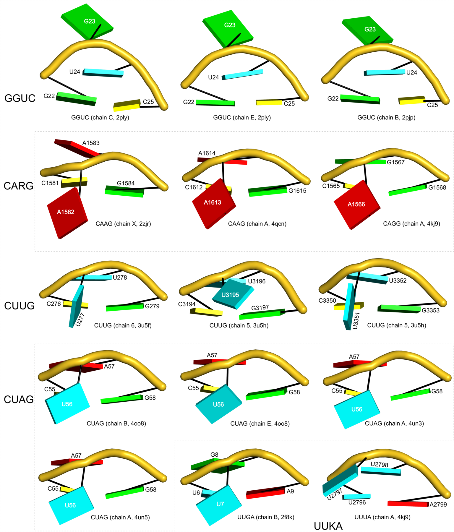
Quote
Figure S9: Images of 15 diloops (GGUC, CARG, CUUG, CUAG, and UUKA) identified by DSSR in the NR3A-dataset. The diloops can be categorized into five groups by base sequence: GGUC, where the second position G is flipped away from the closing pair; CARG, where the second position A is extruded into the minor-groove side of the closing pair; CUUG, which shows structural variations in the three crystallographic examples and differences from their NMR solution counterpart (PDB id: 1rng, Figure 6C); CUAG, where all four cases occur in Cas9 complexes either without (PDB id: 4oo8) or with (PDB ids: 4un3 and 4un5) a protospacer adjacent motif; and UUKA, where the two cases are quite distinct.
The file 'all-diloops.txt' contains a collection of all diloops identified by DSSR in the non-redundant dataset of RNA crystal structures solved at 3.0 Å or better resolution (referred to as the NR3A-dataset in the paper, release 1.89 on 5 December 2014). The corresponding file 'all-diloops.pdb' contains all the 15 diloops in a MODEL/ENDMDL ensemble where each one is re-oriented with the minor-groove edge of the closing Watson-Crick base pair facing the viewer. So for the diloop from chain B of 4oo8 (a CRISPR Cas9 ternary complex), which has the following info in 'all-diloops.txt':
Code: [Select]
4oo8 2 nts=4 CUAG B.C55,B.U56,B.A57,B.G58 C3',C2',C2',C3' anti,anti,anti,antithe transformation option is: --frame=B.55:wc+edge. The transformed diloops (stored in 'all-diloops.pdb') now share the same view for direct comparison.
With all the diloops in proper orientation, the following scripts ("tasks") generates each diloop image in png format.
Code: Bash
- ex_str -1 all-diloops.pdb 2f8k-1-UUGA.pdb
- x3dna-dssr -i=2f8k-1-UUGA.pdb -o=2f8k-1-UUGA-blocks.r3d --block-file
- pymol -qkc 2f8k-1-UUGA.pml
- convert -trim +repage -border 10 -bordercolor white 2f8k-1-UUGA-pymol.png 2f8k-1-UUGA.png
- ex_str -2 all-diloops.pdb 2pjp-1-GGUC.pdb
- x3dna-dssr -i=2pjp-1-GGUC.pdb -o=2pjp-1-GGUC-blocks.r3d --block-file
- pymol -qkc 2pjp-1-GGUC.pml
- convert -trim +repage -border 10 -bordercolor white 2pjp-1-GGUC-pymol.png 2pjp-1-GGUC.png
- ex_str -3 all-diloops.pdb 2ply-1-GGUC.pdb
- x3dna-dssr -i=2ply-1-GGUC.pdb -o=2ply-1-GGUC-blocks.r3d --block-file
- pymol -qkc 2ply-1-GGUC.pml
- convert -trim +repage -border 10 -bordercolor white 2ply-1-GGUC-pymol.png 2ply-1-GGUC.png
- ex_str -4 all-diloops.pdb 2ply-2-GGUC.pdb
- x3dna-dssr -i=2ply-2-GGUC.pdb -o=2ply-2-GGUC-blocks.r3d --block-file
- pymol -qkc 2ply-2-GGUC.pml
- convert -trim +repage -border 10 -bordercolor white 2ply-2-GGUC-pymol.png 2ply-2-GGUC.png
- ex_str -5 all-diloops.pdb 2zjr-40-CAAG.pdb
- x3dna-dssr -i=2zjr-40-CAAG.pdb -o=2zjr-40-CAAG-blocks.r3d --block-file
- pymol -qkc 2zjr-40-CAAG.pml
- convert -trim +repage -border 10 -bordercolor white 2zjr-40-CAAG-pymol.png 2zjr-40-CAAG.png
- ex_str -6 all-diloops.pdb 3u5f-7-CUUG.pdb
- x3dna-dssr -i=3u5f-7-CUUG.pdb -o=3u5f-7-CUUG-blocks.r3d --block-file
- pymol -qkc 3u5f-7-CUUG.pml
- convert -trim +repage -border 10 -bordercolor white 3u5f-7-CUUG-pymol.png 3u5f-7-CUUG.png
- ex_str -7 all-diloops.pdb 3u5h-69-CUUG.pdb
- x3dna-dssr -i=3u5h-69-CUUG.pdb -o=3u5h-69-CUUG-blocks.r3d --block-file
- pymol -qkc 3u5h-69-CUUG.pml
- convert -trim +repage -border 10 -bordercolor white 3u5h-69-CUUG-pymol.png 3u5h-69-CUUG.png
- ex_str -8 all-diloops.pdb 3u5h-72-CUUG.pdb
- x3dna-dssr -i=3u5h-72-CUUG.pdb -o=3u5h-72-CUUG-blocks.r3d --block-file
- pymol -qkc 3u5h-72-CUUG.pml
- convert -trim +repage -border 10 -bordercolor white 3u5h-72-CUUG-pymol.png 3u5h-72-CUUG.png
- ex_str -9 all-diloops.pdb 4kj9-40-CAGG.pdb
- x3dna-dssr -i=4kj9-40-CAGG.pdb -o=4kj9-40-CAGG-blocks.r3d --block-file
- pymol -qkc 4kj9-40-CAGG.pml
- convert -trim +repage -border 10 -bordercolor white 4kj9-40-CAGG-pymol.png 4kj9-40-CAGG.png
- ex_str -10 all-diloops.pdb 4kj9-69-UUUA.pdb
- x3dna-dssr -i=4kj9-69-UUUA.pdb -o=4kj9-69-UUUA-blocks.r3d --block-file
- pymol -qkc 4kj9-69-UUUA.pml
- convert -trim +repage -border 10 -bordercolor white 4kj9-69-UUUA-pymol.png 4kj9-69-UUUA.png
- ex_str -11 all-diloops.pdb 4oo8-2-CUAG.pdb
- x3dna-dssr -i=4oo8-2-CUAG.pdb -o=4oo8-2-CUAG-blocks.r3d --block-file
- pymol -qkc 4oo8-2-CUAG.pml
- convert -trim +repage -border 10 -bordercolor white 4oo8-2-CUAG-pymol.png 4oo8-2-CUAG.png
- ex_str -12 all-diloops.pdb 4oo8-6-CUAG.pdb
- x3dna-dssr -i=4oo8-6-CUAG.pdb -o=4oo8-6-CUAG-blocks.r3d --block-file
- pymol -qkc 4oo8-6-CUAG.pml
- convert -trim +repage -border 10 -bordercolor white 4oo8-6-CUAG-pymol.png 4oo8-6-CUAG.png
- ex_str -13 all-diloops.pdb 4qcn-37-CAAG.pdb
- x3dna-dssr -i=4qcn-37-CAAG.pdb -o=4qcn-37-CAAG-blocks.r3d --block-file
- pymol -qkc 4qcn-37-CAAG.pml
- convert -trim +repage -border 10 -bordercolor white 4qcn-37-CAAG-pymol.png 4qcn-37-CAAG.png
- ex_str -14 all-diloops.pdb 4un3-2-CUAG.pdb
- x3dna-dssr -i=4un3-2-CUAG.pdb -o=4un3-2-CUAG-blocks.r3d --block-file
- pymol -qkc 4un3-2-CUAG.pml
- convert -trim +repage -border 10 -bordercolor white 4un3-2-CUAG-pymol.png 4un3-2-CUAG.png
- ex_str -15 all-diloops.pdb 4un5-2-CUAG.pdb
- x3dna-dssr -i=4un5-2-CUAG.pdb -o=4un5-2-CUAG-blocks.r3d --block-file
- pymol -qkc 4un5-2-CUAG.pml
- convert -trim +repage -border 10 -bordercolor white 4un5-2-CUAG-pymol.png 4un5-2-CUAG.png
- For the aforementioned diloop from chain B of 4oo8, the png image is named 4oo8-2-CUAG.png (see the script above) and is shown below:
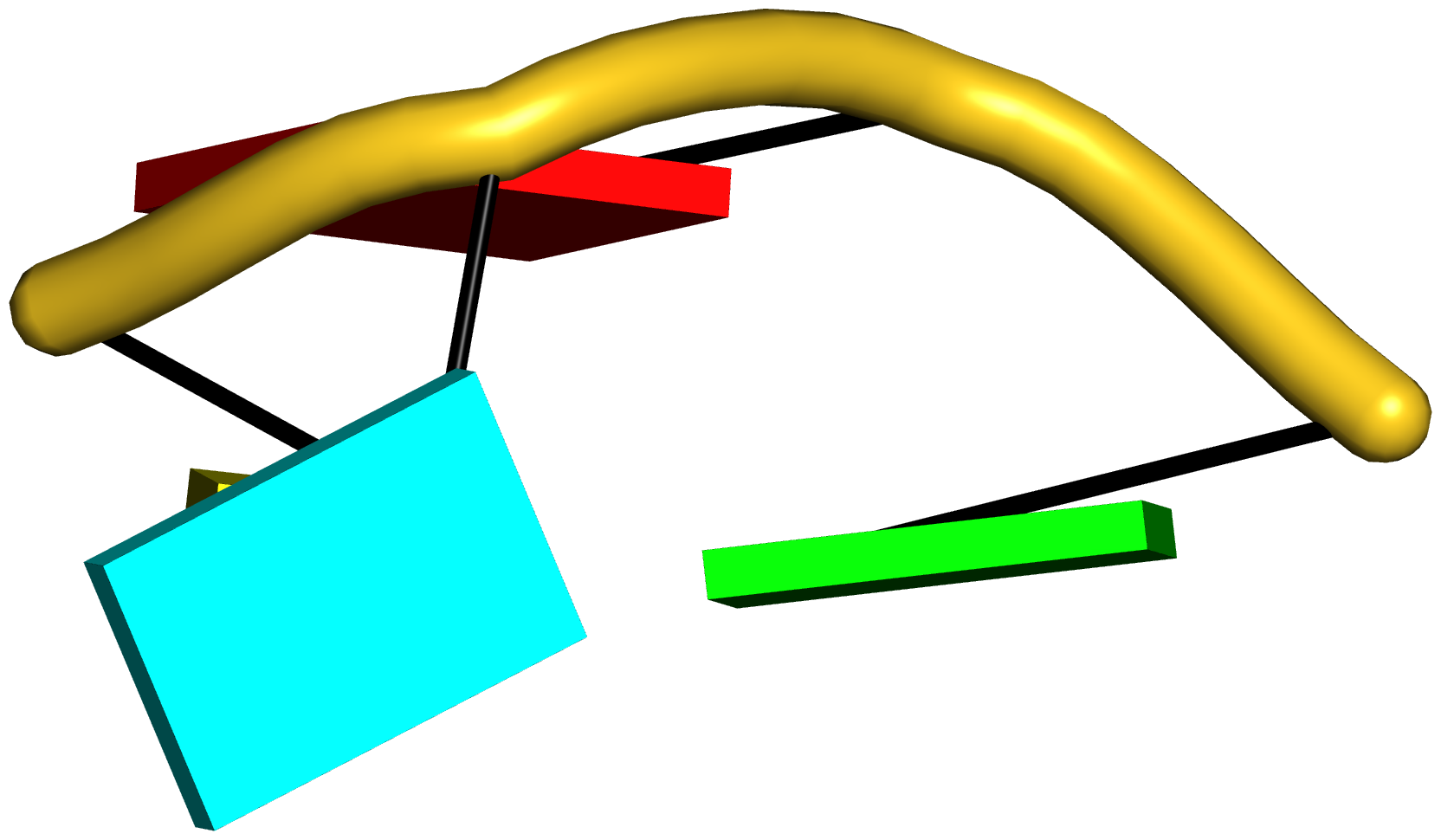 .
. - The ex_str utility program is from the 3DNA distribution. It is used to extract a specific model from a MODEL/ENDMDL ensemble.
- The --block-file option generates a .r3d file with base rectangular blocks for rendering in PyMOL.
- The convert program is from ImageMagick that is used here to trim extra white boundaries.
- The 15 diloop-png images were combined using InkScape, and annotated, to get the final illustration.
- For completeness, here is the tarball file containing all the data files and the script ("tasks"): supp-fig9-diloops.tar.gz
73
DSSR-NAR paper / Supplementary Figure 8 -- 2nd structure diagram of CRISPR RNA-DNA hybrid (4oo8)
« on: July 08, 2015, 01:14:35 am »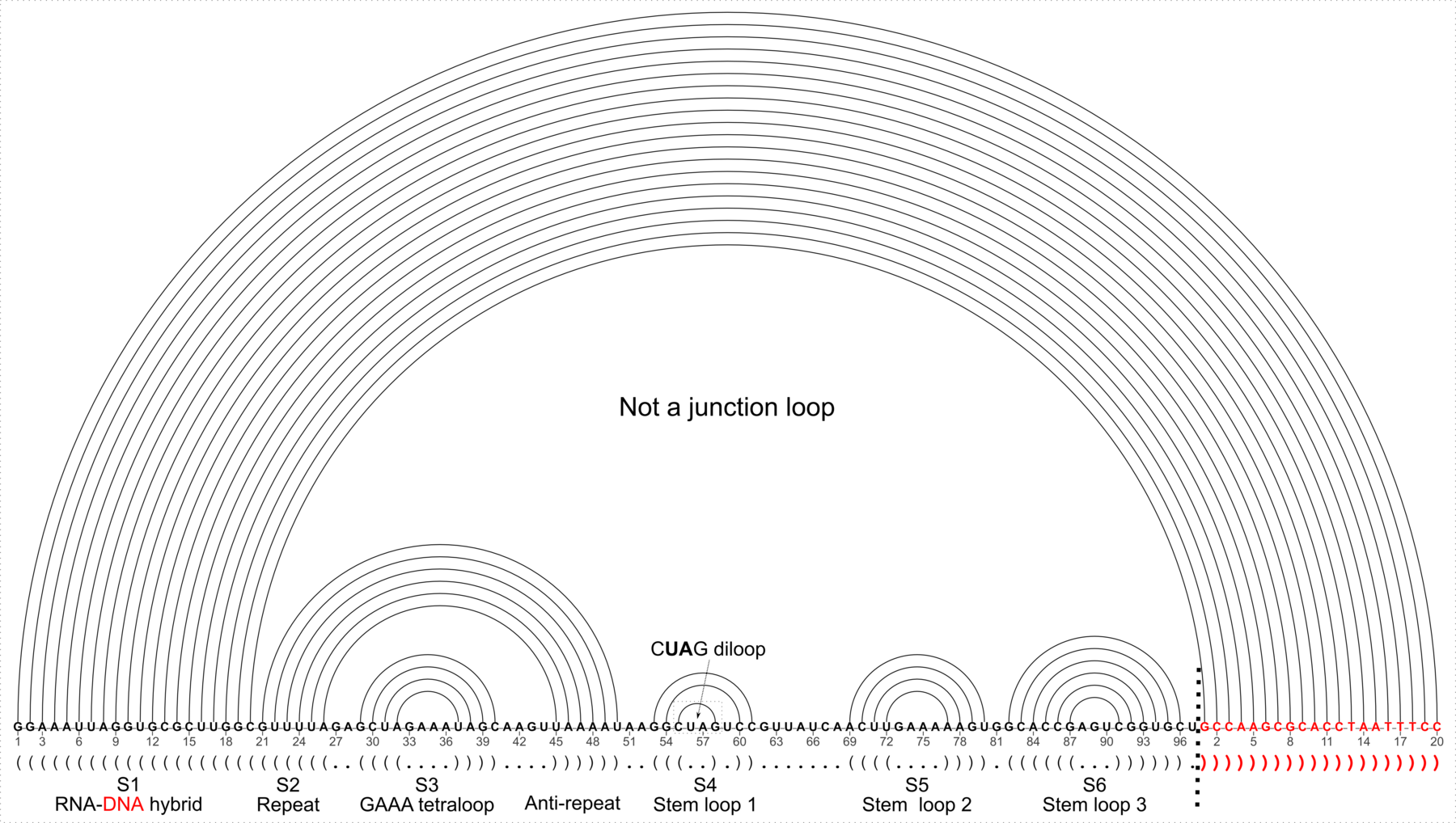
Quote
Figure S8: The linear (arc) secondary structure diagram of the RNA-DNA hybrid structure in the CRISPR Cas9-sgRNA-DNA ternary complex (PDB id: 4oo8), annotated with DSSR-derived dot-bracket notation and key structural elements. The target DNA base se- quence is colored red, and the chain switch from sgRNA to DNA is marked by the dotted vertical line. DSSR detects no junction loops in this hybrid structure because of the chain break.
Starting from "4oo8.pdb" downloaded from RCSB PDB, here is the script to get the secondary structure files to be rendered using VARNA.
Code: [Select]
pdb_frag B 1:97 C 1:20 4oo8.pdb 4oo8-BC.pdb
x3dna-dssr -i=4oo8-BC.pdb -o=4oo8-BC.out --prefix=4oo8-BC
The DSSR-derived 4oo8-BC-2ndstrs.ct file retains residue numbers as in the original PDB file. Here the RNA chain is numbered from 1 to 97, whilst the DNA chain is numbered from 1 to 20. The .ct file, as shown below, is used for rendering with VARNA.
Code: [Select]
  117 ENERGY = 0.0 [4oo8-BC] -- secondary structure derived by DSSR
    1 G     0     1   117     1
    2 G     1     2   116     2
    3 A     2     3   115     3
    4 A     3     4   114     4
    5 A     4     5   113     5
    6 U     5     6   112     6
    7 U     6     7   111     7
    8 A     7     8   110     8
    9 G     8     9   109     9
   10 G     9    10   108    10
   11 U    10    11   107    11
   12 G    11    12   106    12
   13 C    12    13   105    13
   14 G    13    14   104    14
   15 C    14    15   103    15
   16 U    15    16   102    16
   17 U    16    17   101    17
   18 G    17    18   100    18
   19 G    18    19    99    19
   20 C    19    20    98    20
   21 G    20    21    50    21
   22 U    21    22    49    22
   23 U    22    23    48    23
   24 U    23    24    47    24
   25 U    24    25    46    25
   26 A    25    26    45    26
   27 G    26    27     0    27
   28 A    27    28     0    28
   29 G    28    29    40    29
   30 C    29    30    39    30
   31 U    30    31    38    31
   32 A    31    32    37    32
   33 G    32    33     0    33
   34 A    33    34     0    34
   35 A    34    35     0    35
   36 A    35    36     0    36
   37 U    36    37    32    37
   38 A    37    38    31    38
   39 G    38    39    30    39
   40 C    39    40    29    40
   41 A    40    41     0    41
   42 A    41    42     0    42
   43 G    42    43     0    43
   44 U    43    44     0    44
   45 U    44    45    26    45
   46 A    45    46    25    46
   47 A    46    47    24    47
   48 A    47    48    23    48
   49 A    48    49    22    49
   50 U    49    50    21    50
   51 A    50    51     0    51
   52 A    51    52     0    52
   53 G    52    53    61    53
   54 G    53    54    60    54
   55 C    54    55    58    55
   56 U    55    56     0    56
   57 A    56    57     0    57
   58 G    57    58    55    58
   59 U    58    59     0    59
   60 C    59    60    54    60
   61 C    60    61    53    61
   62 G    61    62     0    62
   63 U    62    63     0    63
   64 U    63    64     0    64
   65 A    64    65     0    65
   66 U    65    66     0    66
   67 C    66    67     0    67
   68 A    67    68     0    68
   69 A    68    69    80    69
   70 C    69    70    79    70
   71 U    70    71    78    71
   72 U    71    72    77    72
   73 G    72    73     0    73
   74 A    73    74     0    74
   75 A    74    75     0    75
   76 A    75    76     0    76
   77 A    76    77    72    77
   78 A    77    78    71    78
   79 G    78    79    70    79
   80 U    79    80    69    80
   81 G    80    81     0    81
   82 G    81    82    96    82
   83 C    82    83    95    83
   84 A    83    84    94    84
   85 C    84    85    93    85
   86 C    85    86    92    86
   87 G    86    87    91    87
   88 A    87    88     0    88
   89 G    88    89     0    89
   90 U    89    90     0    90
   91 C    90    91    87    91
   92 G    91    92    86    92
   93 G    92    93    85    93
   94 U    93    94    84    94
   95 G    94    95    83    95
   96 C    95    96    82    96
   97 U    96    97     0    97
   98 G     0    98    20     1
   99 C    98    99    19     2
  100 C    99   100    18     3
  101 A   100   101    17     4
  102 A   101   102    16     5
  103 G   102   103    15     6
  104 C   103   104    14     7
  105 G   104   105    13     8
  106 C   105   106    12     9
  107 A   106   107    11    10
  108 C   107   108    10    11
  109 C   108   109     9    12
  110 T   109   110     8    13
  111 A   110   111     7    14
  112 A   111   112     6    15
  113 T   112   113     5    16
  114 T   113   114     4    17
  115 T   114   115     3    18
  116 C   115   116     2    19
117 C 116 0 1 20Note:- Among the two copies of the tertiary complex, the RNA chain B and DNA chain C are extracted to file 4oo8-BC.pdb for analysis.
- Among the three files (4oo8-BC-2ndstrs.bpseq, 4oo8-BC-2ndstrs.ct and 4oo8-BC-2ndstrs.dbn) for secondary structure representations, the .ct format is more informative.
- There are many options for rendering a secondary structure in VARNA. Here the linear form is used, with a number-period of three, and simple 'line' base-pair style etc.
- The VARNA-exported .svg file is then read into InkSkype for further revisions and annotation, including alignment of the dot-bracket notation with the base sequence, and labeling the six stems and the CUAG diloop etc.
- For completeness, here is the tarball file containing all the data files and the script ("tasks"): supp-fig8-crispr-4oo8.tar.gz
74
DSSR-NAR paper / Supplementary Figure 6 -- DSSR-identified k-turn in the SAM-I riboswitch
« on: July 07, 2015, 05:34:29 pm »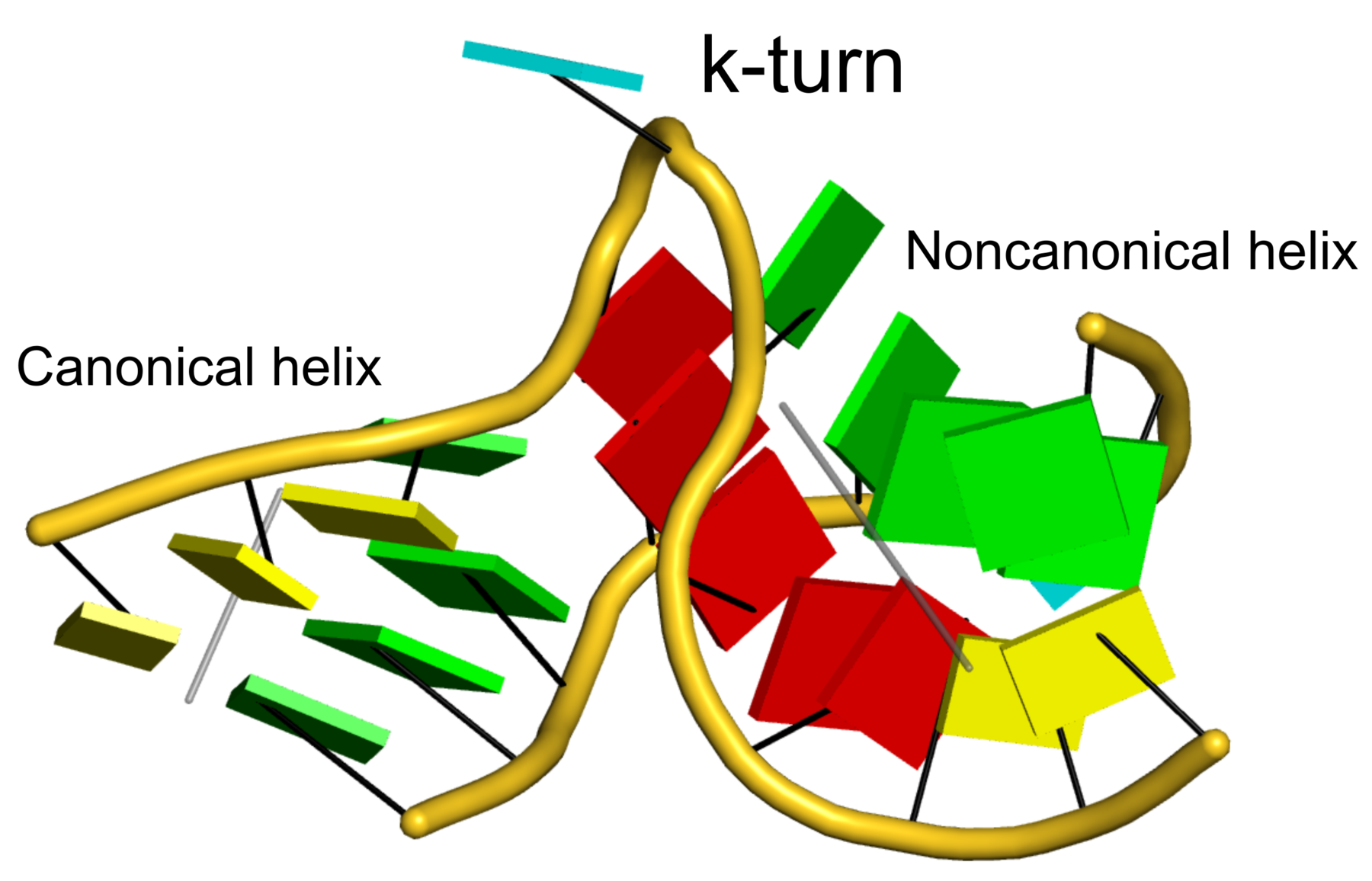
Quote
Figure S6: The k-turn identified by DSSR in the SAM-I riboswitch (PDB id: 2gis). Base-stacking interactions are interrupted around the k-turn even though the backbone is continuous along each strand. Thus DSSR assigns two helices (depicted by gray lines), the canonical helix on the left, and the noncanonical one on the right.
Starting from 2gis.pdb downloaded from the RCSB website, here is the complete script.
Code: Bash
- x3dna-dssr -i=2gis.pdb -o=2gis.out --prefix=2gis
- \cp 2gis-Kturns.pdb 2gis-kturn.pdb
- x3dna-dssr -i=2gis-kturn.pdb -o=2gis-kturn.out --helical-axis
- \cp dssr-helicalAxes.pdb 2gis-kturn-helices.pdb
- x3dna-dssr -i=2gis-kturn.pdb -o=2gis-kturn-blocks.r3d --block-file
- pymol -qkc 2gis-kturn.pml
- convert -trim +repage -border 10 -bordercolor white 2gis-kturn-pymol.png 2gis-kturn.png
Note:
- The --helical-axis option outputs the best-fitted helical axes in file "dssr-helicalAxes.pdb".
- The --block-file option creates a .r3d file with bases (or Watson-Crick base pairs) in rectangular block represention.
- The convert program is from ImageMagick that is used here to trim extra white boundaries.
- The png image was annotated using InkScape for the final illustration.
- For completeness, here is the tarball file containing all the data files and the script ("tasks"): supp-fig6-kturn-2gis.tar.gz
75
DSSR-NAR paper / Supplementary Figure 5 -- characterizing junction loops in twister ribozyme
« on: July 07, 2015, 01:56:51 pm »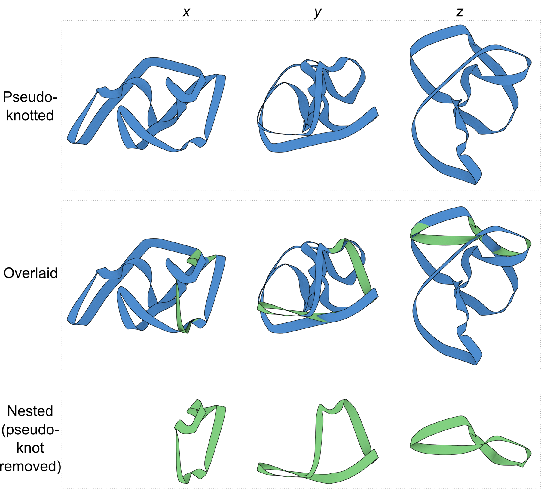
Quote
Figure S5: Ribbon representations of the junction loop in the env22 twister ribozyme (PDB id: 4rge). The ribbons are defined in terms of the C1′ and P atoms of the nucleotides that make up the junction loop. Inclusion of pseudoknots in the analysis of the structure reveals a [4,2,2,0,1,3,0,0,1,1] ten-way junction and a ribbon that follows a super-coiled pathway, with a linking number of three (blue, top row). Upon pseudoknot removal, only a [2,1,3] three-way junction and a ribbon with a simple relaxed circular configuration remain (green, bottom row). The overlap of the two junction loops in the middle row clearly shows that the over-simplified three-way junction spans only a small portion of the ten-way loop. The ribbons are shown in three projections: down the x-axis (left column), the y-axis (middle column), and the z-axis (right column). The images were kindly generated by Dr. Nicolas Clauvelin using the approach described in ref. 49.
Note:
- I provided Dr. Nicolas Clauvelin these two files: twister-pknot-jct.pdb for the ten-way junction, and a simplified version twister-nested-jct.pdb for the pseudoknots-removed three-way junction.
- Dr. Nicolas Clauvelin generated the ribbon diagrams of the pseudo-knotted/free junction loops and their overlaid version, each in three projections for a total of 9 files.
- The nine png images were combined using InkScape, and annotated, to get the final illustration.
- For completeness, here is the tarball file containing all the data files: supp-fig5-twister-4rge.tar.gz
Funded by the NIH R24GM153869 grant on X3DNA-DSSR, an NIGMS National Resource for Structural Bioinformatics of Nucleic Acids
Created and maintained by Dr. Xiang-Jun Lu, Department of Biological Sciences, Columbia University