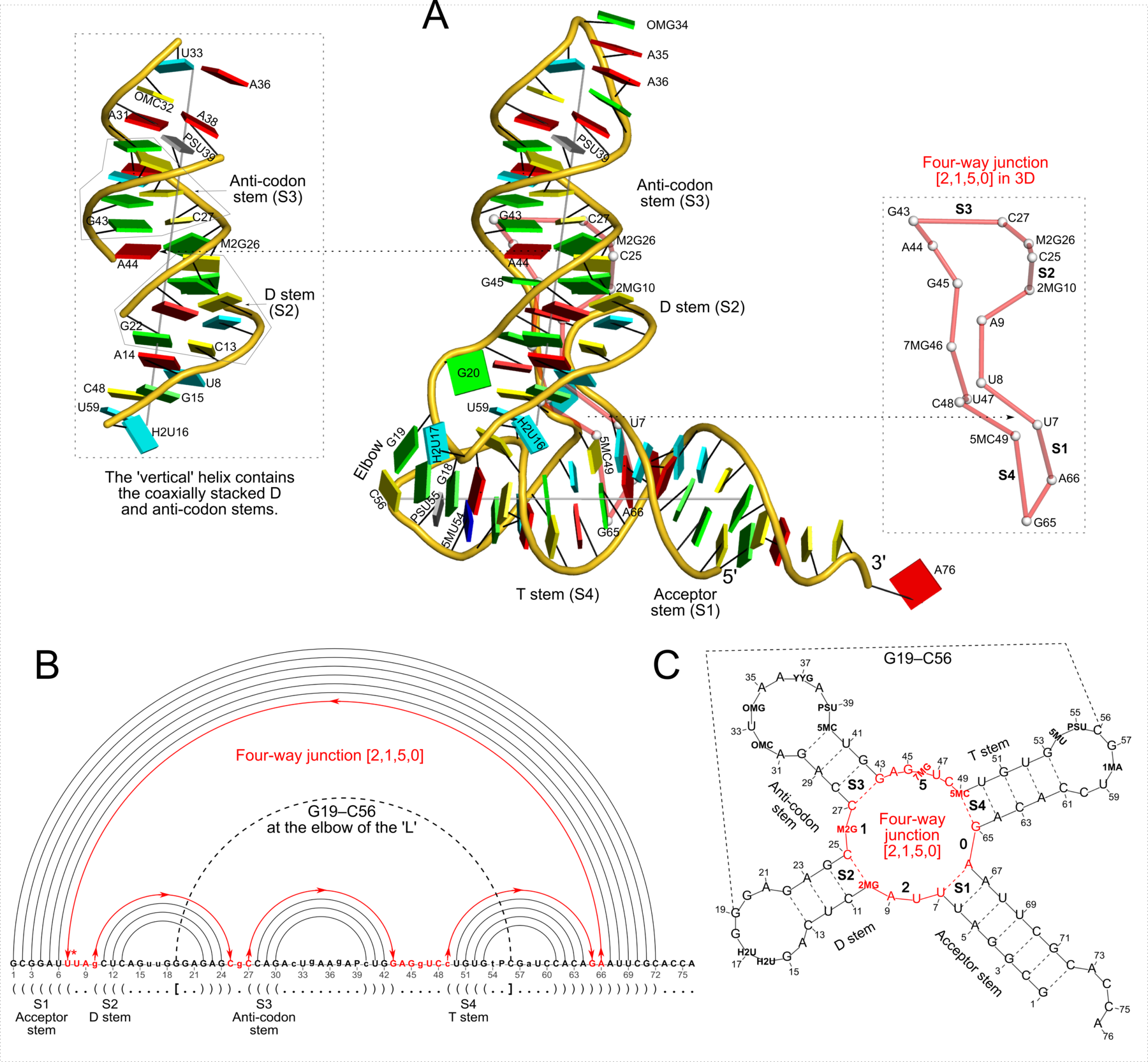
Figure 2: DSSR captures well-known features and provides a new perspective on the classic yeast tRNAPhe structure (PDB id: 1ehz (46)). (A) The software automatically detects the four stems and the two helices that form the L-shaped molecule, depicted here in cartoon-block representation (center). Whereas the helices may include all types of base pairs and backbone breaks, the stems comprise only canonical pairs with continuous backbones. Note the coaxial stacking of the D and anti-codon stems and the noncanonical features of the composite helix (represented by a gray line, left). The red ‘circle’, overlaid on the central image and detailed to the right, reveals the 3D pathway along the [2,1,5,0] four-way junction loop. (B) The dot-bracket notation derived by DSSR serves as input for the depicted linear (arc) representation of secondary structure. The bases comprising the four-way junction loop (red) run in sequential order from U7 (*) following the arrows to the right and returning along the outer A66→U7 arc. The pseudoknotted G19–C56 pair (with matched []) is noted by the dashed arc. (C) Both the four-way junction (red) and the three hairpin loops follow ‘circular’ routes within the traditional cloverleaf representation of tRNA. Here the 14 modified nucleotides are represented by three-letter codes. The 3D images were created using PyMOL (A-red; C-yellow; G-green; T-blue; U-cyan; pseudouridine P-gray), the 2D diagrams using VARNA, and the annotations using Inkscape.
It takes many steps and great attention to details to generate the above figure, even though the basic idea is quite simple. The following script (in file '
tasks') takes advantage of 3DNA, PyMOL, VARNA, ImageMagick, Inkscape and some previously undocumented DSSR options. It is
not the raw script originally used to create Figure 2 of the DSSR-NAR paper. For easy followup, the script has been made more self-contained, at the expense of apparent
repetition of commands and PyMOL settings in various
.pml files.
For understanding of the script, detailed notes are provided below for each major step. The 3D images in .png format and secondary structure diagrams in .svg format are combined and annotated using Inkscape. Great care has been taken to ensure the accuracy of details and quality of the figure. By and large, Figures 3-6 and Supplementary Figures 1-9 follow the same convention.
# Step #1 -- reorient tRNA into the classic "L" shape
x3dna-dssr -i=1ehz.pdb -o=1ehz.out --more --prefix=1ehz
pdb_frag A 1:76 1ehz.pdb 1ehz-nts.pdb
# extract the two helical axes from 1ehz.out to file: 1ehz.rot1
# then reorient the structure into the "L" shape: 1ehz.rot2
rotate_mol -t=1ehz.rot1 1ehz-nts.pdb 1ehz-rot1.pdb
rotate_mol -r=1ehz.rot2 1ehz-rot1.pdb 1ehz-ok.pdb
# Step #2 -- get the cartoon-block representation with the two
# ls-fitted helical axes.
x3dna-dssr -i=1ehz-ok.pdb --helical-axis -o=temp
\mv dssr-helicalAxes.pdb 1ehz-ok-helices.pdb
x3dna-dssr -i=1ehz-ok.pdb --block-file -o=1ehz-ok-blocks.r3d
# Step #3 -- simplified representation of the [2,1,5,0] 4-way junction in 3D
# -- note the --raw-xyz option: it keeps the original coordinates
x3dna-dssr -i=1ehz-ok.pdb --raw-xyz --simple-junction -o=temp
\mv dssr-simplifiedJcts.pdb 1ehz-ok-jct.pdb
# see file: 1ehz-ok-jct.pml
pymol -qkc 1ehz-ok-jct.pml
convert -trim +repage -border 10 -bordercolor white 1ehz-ok-jct-pymol.png 1ehz-ok-jct.png
# see file: 1ehz-ok-full.pml (cartoon-block with the schematic junction overlaid)
pymol -qkc 1ehz-ok-full.pml
convert -trim +repage -border 10 -bordercolor white 1ehz-ok-full-pymol.png 1ehz-ok-full.png
# Step #4 -- illustration of 'vertical' helix of the "L", composed of
# anti-codon and D stems, coaxially stacked around M2G26-A44
x3dna-dssr -i=1ehz-ok.pdb --raw-xyz -o=temp
ex_str -2 dssr-helices.pdb 1ehz-ok-h2.pdb
x3dna-dssr -i=1ehz-ok-h2.pdb --helical-axis -o=temp
\mv dssr-helicalAxes.pdb 1ehz-ok-h2-helices.pdb
x3dna-dssr -i=1ehz-ok-h2.pdb --block-file -o=1ehz-ok-h2-blocks.r3d
# see file: 1ehz-ok-h2.pml
pymol -qkc 1ehz-ok-h2.pml
convert -trim +repage -border 10 -bordercolor white 1ehz-ok-h2-pymol.png 1ehz-ok-h2.png
The helix containing the acceptor/T stems is put "horizontal", and the one with D/anti-codon stems "vertical".
- The DSSR --prefix option gives rise to three files 1ehz-2ndstrs.ct, 1ehz-2ndstrs.dbn and 1ehz-2ndstrs.bpseq for the representations of the secondary structure. Overall, the .ct format is more informative, and .dbn most compact. Any of the three files can be loaded directly into VARNA for the visualization of the secondary structure. There are many settings one can play with in VARNA. In Panel B and C, I used the simple "Line" BP style, set number period to 3, clicked "Toggle draw bases" etc. In VARNA, Panel B is in the so-called "Linear" style, and Panel C in "Radiate" style. The VARNA secondary structure diagrams are exported into .svg format for further annotation in Inkscape.
- The first DSSR run (line no.2) specifies the --more option to output detailed output of the two helical axes in file 1ehz.out
  helix#1[2] bps=15
      strand-1 5'-GCGGAUUcUGUGtPC-3'
       bp-type    ||||||||||||..|
      strand-2 3'-CGCUUAAGACACaGG-5'
      helix-form  AA....xAAAAxx.
    helical-rise:   3.00(0.90) *
    helical-radius: 8.88(1.77) *
    helical-axis:    0.617     0.739    -0.269 *

  helix#2[2] bps=15
      strand-1 5'-AAPcUGGAgCUCAGu-3'
       bp-type    ...||||.||||...
      strand-2 3'-UcAGACCgCGAGUCU-5'
      helix-form  x..AAAAxAA.xxx
    helical-rise:   3.07(1.12) *
    helical-radius: 8.89(2.35) *
    helical-axis:    0.071     0.444     0.893 *
- The pdb_frag utility program from 3DNA (in folder $X3DNA/perl_scripts) extracts all the 76 nucleotides on chain A of 1ehz.pdb to 1ehz-nts.pdb. The script is included here for completeness.
- The vectors of the two helical axes are collected into file 1ehz.rot1 to set the structure (using rotate_mol) into an orientation shown below. See also "Recipe no. 4: command-line script to illustrate the three helices in a four-way DNA-RNA junction" of the 2008 3DNA Nature Protocols paper.
     1  # x-, y-, z-axes row-rise
      0.000    0.000    0.000   # translation
      0.617    0.739   -0.269   # h1
      0.071    0.444    0.893   # h2
      0.000   0.000   1.000   # z: can be anything
- The second run of rotate_mol put the tRNA (1ehz) into its final orientation (1ehz-ok.pdb). The content of 1ehz.rot2
is as below:
by rotation y 180
by rotation x 180
The transformed PDB coordinate file 1ehz-ok.pdb is the starting point of all the following illustrations.
Step #2: -- get the cartoon-block representation with the two least-squares-fitted helical axes.
Step #3 -- simplified representation of the [2,1,5,0] 4-way junction in 3D
- The DSSR --raw-xyz option makes the auxiliary PDB files in the original coordinates instead of in certain new reference frames. For example, by default, the dssr-pairs.pdb file has each pair in the its own reference frame (top view) that enables easy comparison and visualization. Here, the --raw-xyz option is used to ensure a direct comparison of the 4-way junction loop in isolation vs that overlaid within the whole tRNA structure (1ehz-ok.pdb). The default junction file dssr-junctions.pdb is renamed 1ehz-ok-4wj.pdb for easy reference.
- The DSSR --simple-junction option produces another auxiliary file, named dssr-simplifiedJcts.pdb by default, and renamed 1ehz-ok-jct.pdb for easy reference. The file contains the atomic coordinates of C1′ atoms of the 4-way junction loop, with content shown below. Note that the nucleotides are in proper sequential order.
MODEL        1
REMARK    model=1  nts=16
REMARK    4-way junction: nts=16; [2,1,5,0]; linked by [#1,#2,#3,#4]
ATOM      1  C1'   U A   7     -65.936 -49.847  29.027  1.00 37.23           C
ATOM      2  C1'   U A   8     -72.670 -44.818  30.530  1.00 30.28           C
ATOM      3  C1'   A A   9     -72.606 -37.344  27.403  1.00 28.79           C
HETATM    4  C1' 2MG A  10     -66.888 -33.680  24.426  1.00 44.62           C
ATOM      5  C1'   C A  25     -66.556 -29.785  34.413  1.00 51.93           C
HETATM    6  C1' M2G A  26     -66.983 -28.143  29.356  1.00 46.92           C
ATOM      7  C1'   C A  27     -70.138 -25.556  25.591  1.00 48.68           C
ATOM      8  C1'   G A  43     -80.779 -25.396  27.582  1.00 46.94           C
ATOM      9  C1'   A A  44     -78.474 -28.381  24.234  1.00 54.14           C
ATOM     10  C1'   G A  45     -75.498 -32.895  24.403  1.00 45.24           C
HETATM   11  C1' 7MG A  46     -76.230 -40.483  24.555  1.00 39.69           C
ATOM     12  C1'   U A  47     -74.362 -46.762  19.557  1.00 50.55           C
ATOM     13  C1'   C A  48     -75.266 -47.135  28.377  1.00 27.98           C
HETATM   14  C1' 5MC A  49     -68.564 -51.174  23.872  1.00 33.10           C
ATOM     15  C1'   G A  65     -67.234 -61.378  20.695  1.00 42.23           C
ATOM     16  C1'   A A  66     -64.217 -56.459  21.032  1.00 40.50           C
CONECT    1   16    2
CONECT    2    1    3
CONECT    3    2    4
CONECT    4    3    5
CONECT    5    4    6
CONECT    6    5    7
CONECT    7    6    8
CONECT    8    7    9
CONECT    9    8   10
CONECT   10    9   11
CONECT   11   10   12
CONECT   12   11   13
CONECT   13   12   14
CONECT   14   13   15
CONECT   15   14   16
CONECT   16   15    1
ENDMDL
- The 4-way junction in a simplified representation is ray-traced with PyMOL based on 1ehz-ok-jct.pml. The style of the 4-way junction is controlled by various PyMOL settings, as shown below.
load 1ehz-ok-jct.pdb, jct
hide everything, jct

set sphere_color, white, jct
set sphere_scale, 0.36, jct
show spheres, jct

set stick_radius, 0.3, jct
set stick_color, red, jct
set stick_transparency, 0.46, jct
show sticks, jct
# -----------------------------------------

bg_color white

util.cbaw
set sphere_quality, 4
set stick_quality, 16

# PyMOL FAQ recommendations
set depth_cue, 0
set ray_trace_fog, 0

set ray_shadow, off
set orthoscopic, 1

set antialias, 1
# cannot be: zoom complete, 1
zoom complete=1
# -----------------------------------------

ray 1800
png 1ehz-ok-jct-pymol.png
The PyMOL options -qkc is used to generate file 1ehz-ok-jct-pymol.png from command line. Note the extra white space around the image (see below).
- The convert command from the popular ImageMagick package is employed simply to crop the extra white space around PyMOL-generated png image.
- The 1ehz-ok-full.pml PyMOL script combines all the components (backbone cartoon with ladder for bases, colored base rectangular blocks, gray helical axes, and the overlaid schematic 4-way junction loop) to generate the main part of panel A of the figure. See below:
Step #4 -- illustration of 'vertical' helix of the L-shaped tRNA
- Note the three options --raw-xyz, --helical-axis, and --block-file mentioned above.
- The PyMOL script file is 1ehz-ok-h2.pml, and the final generated image is shown below:


 Topic: Figure 2 -- analysis of the yeast phenylalanine tRNA (1ehz) (Read 61599 times)